Every problem in the chapter beside the book’s answer, a chapter at a time as you scroll.
Chapter 2: Descriptive Statistics
65 problems · 26 figures2-1 §2.1 source ↗
For each of the following data sets, create a stemplot and identify any outliers.
The miles-per-gallon ratings for 30 cars are shown below (lowest to highest):
19, 19, 19, 20, 21, 21, 25, 25, 25, 26, 26, 28, 29, 31, 31, 32, 32, 33, 34, 35, 36, 37, 37, 38, 38, 38, 38, 41, 43, 43.
Answer
| Stem | Leaf |
|---|---|
| 1 | 9 9 9 |
| 2 | 0 1 1 5 5 5 6 6 8 9 |
| 3 | 1 1 2 2 3 4 5 6 7 7 8 8 8 8 |
| 4 | 1 3 3 |
| Stem | Leaf |
|---|---|
| 1 | 9 9 9 |
| 2 | 0 1 1 5 5 5 6 6 8 9 |
| 3 | 1 1 2 2 3 4 5 6 7 7 8 8 8 8 |
| 4 | 1 3 3 |
2-3 §2.1 source ↗
For each of the following data sets, create a stemplot and identify any outliers.
The data are the prices of different laptops at an electronics store. Round each value to the nearest 10.
249, 249, 260, 265, 265, 280, 299, 299, 309, 319, 325, 326, 350, 350, 350, 365, 369, 389, 409, 459, 489, 559, 569, 570, 610
Answer
| Stem | Leaf |
|---|---|
| 2 | 5 5 6 7 7 8 |
| 3 | 0 0 1 2 3 3 5 5 5 7 7 9 |
| 4 | 1 6 9 |
| 5 | 6 7 7 |
| 6 | 1 |
| Stem | Leaf |
|---|---|
| 2 | 5 5 6 7 7 8 |
| 3 | 0 0 1 2 3 3 5 5 5 7 7 9 |
| 4 | 1 6 9 |
| 5 | 6 7 7 |
| 6 | 1 |
2-5 §2.1 source ↗
For the next three exercises, use the data to construct a line graph.
In a survey, 40 people were asked how many times they visited a store before making a major purchase. The results are shown in Table 2.40.
| Number of Times in Store | Frequency |
|---|---|
| 1 | 4 |
| 2 | 10 |
| 3 | 16 |
| 4 | 6 |
| 5 | 4 |
Answer
2-7 §2.1 source ↗
For the next three exercises, use the data to construct a line graph.
Several children were asked how many TV shows they watch each day. The results of the survey are shown in Table 2.42.
| Number of TV Shows | Frequency |
|---|---|
| 0 | 12 |
| 1 | 18 |
| 2 | 36 |
| 3 | 7 |
| 4 | 2 |
Answer
2-9 §2.1 source ↗
For the next three exercises, use the data to construct a line graph.
Using the data from Mrs. Ramirez’s math class supplied in Exercise 2.8, construct a bar graph showing the percentages.
Answer
2-11 §2.1 source ↗
For the next three exercises, use the data to construct a line graph.
Use the data from the David County science competition supplied in Exercise 2.10. Construct a bar graph that shows the county-wide population percentage of students at each school.
Answer
2-13 §2.2 source ↗
| Data Value (Number of Cars) | Frequency | Relative Frequency | Cumulative Relative Frequency |
|---|---|---|---|
Answer
2-15 §2.2 source ↗
| Data Value (Number of Cars) | Frequency | Relative Frequency | Cumulative Relative Frequency |
|---|---|---|---|
Answer
2-17 §2.2 source ↗
| Data Value (Number of Cars) | Frequency | Relative Frequency | Cumulative Relative Frequency |
|---|---|---|---|
Answer
2-19 §2.2 source ↗
| Depth of Hunger | Frequency |
|---|---|
| 230–259 | 21 |
| 260–289 | 13 |
| 290–319 | 5 |
| 320–349 | 7 |
| 350–379 | 1 |
| 380–409 | 1 |
| 410–439 | 1 |
Answer
2-21 §2.2 source ↗
| Sex/Year | 1855 | 1856 | 1857 | 1858 | 1859 | 1860 | 1861 |
| Female | 45,545 | 49,582 | 50,257 | 50,324 | 51,915 | 51,220 | 52,403 |
| Male | 47,804 | 52,239 | 53,158 | 53,694 | 54,628 | 54,409 | 54,606 |
| Total | 93,349 | 101,821 | 103,415 | 104,018 | 106,543 | 105,629 | 107,009 |
| Sex/Year | 1862 | 1863 | 1864 | 1865 | 1866 | 1867 | 1868 | 1869 |
| Female | 51,812 | 53,115 | 54,959 | 54,850 | 55,307 | 55,527 | 56,292 | 55,033 |
| Male | 55,257 | 56,226 | 57,374 | 58,220 | 58,360 | 58,517 | 59,222 | 58,321 |
| Total | 107,069 | 109,341 | 112,333 | 113,070 | 113,667 | 114,044 | 115,514 | 113,354 |
| Sex/Year | 1871 | 1870 | 1872 | 1871 | 1872 | 1827 | 1874 | 1875 |
| Female | 56,099 | 56,431 | 57,472 | 56,099 | 57,472 | 58,233 | 60,109 | 60,146 |
| Male | 60,029 | 58,959 | 61,293 | 60,029 | 61,293 | 61,467 | 63,602 | 63,432 |
| Total | 116,128 | 115,390 | 118,765 | 116,128 | 118,765 | 119,700 | 123,711 | 123,578 |
Answer
2-23 §2.3 source ↗
Listed are 29 ages for Academy Award-winning best actors in order from smallest to largest:
18, 21, 22, 25, 26, 27, 29, 30, 31, 33, 36, 37, 41, 42, 47, 52, 55, 57, 58, 62, 64, 67, 69, 71, 72, 73, 74, 76, 77
a. Find the 40th percentile.
b. Find the 78th percentile.
Answer
a. The 40th percentile is 37 years.
b. The 78th percentile is 70 years.
2-25 §2.3 source ↗
Answer
Jesse graduated 37th out of a class of 180 students. There are 180 – 37 = 143 students ranked below Jesse. There is one rank of 37.
x = 143 and y = 1. (100) = (100) = 79.72. Jesse’s rank of 37 puts him at the 80th percentile.
2-27 §2.3 source ↗
a. For runners in a race, a higher speed means a faster run. Is it more desirable to have a speed with a high or a low percentile when running a race?
b. The 40th percentile of speeds in a particular race is 7.5 miles per hour. Write a sentence interpreting the 40th percentile in the context of the situation.
Answer
a. For runners in a race, it is more desirable to have a high percentile for speed. A high percentile means a higher speed, which is faster.
b. 40 percent of runners ran at speeds of 7.5 miles per hour or less (slower), and 60 percent of runners ran at speeds of 7.5 miles per hour or more (faster).
2-29 §2.3 source ↗
Answer
2-31 §2.3 source ↗
Answer
2-33 §2.3 source ↗
Answer
2-35 §2.3 source ↗
Use Exercise 2.25 to calculate the following values.
Second quartile = median = 50th percentile = ________
Answer
2-37 §2.3 source ↗
Use Exercise 2.25 to calculate the following values.
Interquartile range (IQR) = ________ – ________ = ________
Answer
2-39 §2.3 source ↗
Use Exercise 2.25 to calculate the following values.
70th percentile = ________
Answer
2-41 §2.4 source ↗
Sixty-five randomly selected car salespersons were asked the number of cars they generally sell in one week. Fourteen people answered that they generally sell three cars, 19 generally sell four cars, 12 generally sell five cars, nine generally sell six cars, and 11 generally sell seven cars.
Looking at your box plot, does it appear that the data are concentrated together, spread out evenly, or concentrated in some areas but not in others? How can you tell?
Answer
2-43 §2.5 source ↗
Use the following information to answer the next three exercises: The following data show the lengths of boats moored in a marina. The data are ordered from smallest to largest: 16, 17, 19, 20, 20, 21, 23, 24, 25, 25, 25, 26, 26, 27, 27, 27, 28, 29, 30, 32, 33, 33, 34, 35, 37, 39, 40
Calculate the mean.
Answer
Mean: 16 + 17 + 19 + 20 + 20 + 21 + 23 + 24 + 25 + 25 + 25 + 26 + 26 + 27 + 27 + 27 + 28 + 29 + 30 + 32 + 33 + 33 + 34 + 35 + 37 + 39 + 40 = 738;
= 27.33
2-45 §2.5 source ↗
Use the following information to answer the next three exercises: The following data show the lengths of boats moored in a marina. The data are ordered from smallest to largest: 16, 17, 19, 20, 20, 21, 23, 24, 25, 25, 25, 26, 26, 27, 27, 27, 28, 29, 30, 32, 33, 33, 34, 35, 37, 39, 40
Identify the mode.
Answer
2-47 §2.5 source ↗
Use the following information to answer the next three exercises: Sixty-five randomly selected car salespersons were asked the number of cars they generally sell in one week. Fourteen people answered that they generally sell three cars, 19 generally sell four cars, 12 generally sell five cars, nine generally sell six cars, and 11 generally sell seven cars. Calculate the following.
median = ________
Answer
2-49 §2.6 source ↗
Use the following information to answer the next three exercises. State whether the data are symmetrical, skewed to the left, or skewed to the right.
1, 1, 1, 2, 2, 2, 2, 3, 3, 3, 3, 3, 3, 3, 3, 4, 4, 4, 5, 5
Answer
2-51 §2.6 source ↗
Use the following information to answer the next three exercises. State whether the data are symmetrical, skewed to the left, or skewed to the right.
87, 87, 87, 87, 87, 88, 89, 89, 90, 91
Answer
2-53 §2.6 source ↗
Use the following information to answer the next three exercises. State whether the data are symmetrical, skewed to the left, or skewed to the right.
When the data are symmetrical, what is the typical relationship between the mean and median?
Answer
2-55 §2.6 source ↗
Use the following information to answer the next three exercises. State whether the data are symmetrical, skewed to the left, or skewed to the right.
Describe the shape of this distribution.
Answer
2-57 §2.6 source ↗
Use the following information to answer the next three exercises. State whether the data are symmetrical, skewed to the left, or skewed to the right.
Describe the relationship between the mean and the median of this distribution.
Answer
2-59 §2.6 source ↗
Use the following information to answer the next three exercises. State whether the data are symmetrical, skewed to the left, or skewed to the right.
Describe the relationship between the mode and the median of this distribution.
Answer
2-61 §2.6 source ↗
Use the following information to answer the next three exercises. State whether the data are symmetrical, skewed to the left, or skewed to the right.
Describe the shape of this distribution.
Answer
2-63 §2.6 source ↗
Use the following information to answer the next three exercises. State whether the data are symmetrical, skewed to the left, or skewed to the right.
Describe the relationship between the mean and the median of this distribution.
Answer
2-65 §2.6 source ↗
Use the following information to answer the next three exercises. State whether the data are symmetrical, skewed to the left, or skewed to the right.
Which is the greatest, the mean, the mode, or the median of the data set?
11, 11, 12, 12, 12, 12, 13, 15, 17, 22, 22, 22
Answer
2-67 §2.6 source ↗
Use the following information to answer the next three exercises. State whether the data are symmetrical, skewed to the left, or skewed to the right.
Of the three measures, which tends to reflect skewing the most, the mean, the mode, or the median? Why?
Answer
2-69 §2.7 source ↗
For each of the examples given below, tell whether the differences in outcomes may be explained by measurement variability, natural variability, induced variability, or sampling variability.
Scientists randomly select five groups of 10 women from a population of 1,000 women to record their body fat percentage. The scientists compute the mean body fat percentage from each group. The differences in outcomes may be attributed to which type of variability?
Answer
2-70 §2.7 source ↗
For each of the examples given below, tell whether the differences in outcomes may be explained by measurement variability, natural variability, induced variability, or sampling variability.
A pharmaceutical company randomly assigns participants to one of two groups: one is a control group receiving a placebo, and another is a treatment group receiving a new drug to lower blood pressure. The differences in outcomes may be attributed to which type of variability?
Answer
2-71 §2.7 source ↗
For each of the examples given below, tell whether the differences in outcomes may be explained by measurement variability, natural variability, induced variability, or sampling variability.
Jaiqua and Harold are trying to determine how ramp steepness affects the speed of a ball rolling down the ramp. They measure the time it takes for the ball to roll down ramps of differing slopes. When Jaiqua rolls the ball and Harold works the stopwatch, they get different results than when Harold rolls the ball and Jaiqua works the stopwatch. The differences in outcomes may be attributed to which type of variability?
Answer
2-72 §2.7 source ↗
For each of the examples given below, tell whether the differences in outcomes may be explained by measurement variability, natural variability, induced variability, or sampling variability.
Twenty people begin the same workout program on the same day and continue for three months. During that time, all participants worked out for the same amount of time and did the same number of exercises and repetitions. Each person was weighed at both the beginning and the end of the program. The differences in outcomes regarding the amount of weight lost may be attributed to which type of variability?
Answer
2-73 §2.7 source ↗
Use the following information to answer the next two exercises. The following data are the distances between 20 retail stores and a large distribution center. The distances are in miles.
29, 37, 38, 40, 58, 67, 68, 69, 76, 86, 87, 95, 96, 96, 99, 106, 112, 127, 145, 150
Use a graphing calculator or computer to find the standard deviation and round to the nearest tenth.
Answer
2-75 §2.7 source ↗
Use the following information to answer the next two exercises. The following data are the distances between 20 retail stores and a large distribution center. The distances are in miles.
29, 37, 38, 40, 58, 67, 68, 69, 76, 86, 87, 95, 96, 96, 99, 106, 112, 127, 145, 150
Two baseball players, Fredo and Karl, on different teams wanted to find out who had the higher batting average when compared to his team. Which baseball player had the higher batting average when compared to his team?
| Baseball Player | Batting Average | Team Batting Average | Team Standard Deviation |
|---|---|---|---|
| Fredo | .158 | .166 | .012 |
| Karl | .177 | .189 | .015 |
Answer
For Fredo: z = = –0.67.
For Karl: z = = –.8.
Fredo’s z score of –.67 is higher than Karl’s z score of –.8. For batting average, higher values are better, so Fredo has a better batting average compared to his team.
2-77 §2.7 source ↗
Use the following information to answer the next two exercises. The following data are the distances between 20 retail stores and a large distribution center. The distances are in miles.
29, 37, 38, 40, 58, 67, 68, 69, 76, 86, 87, 95, 96, 96, 99, 106, 112, 127, 145, 150
Find the standard deviation for the following frequency tables using the formula. Check the calculations with the TI 83/84.
a.
b.
c.
| Grade | Frequency |
|---|---|
| 49.5–59.5 | 2 |
| 59.5–69.5 | 3 |
| 69.5–79.5 | 8 |
| 79.5–89.5 | 12 |
| 89.5–99.5 | 5 |
| Daily Low Temperature | Frequency |
|---|---|
| 49.5–59.5 | 53 |
| 59.5–69.5 | 32 |
| 69.5–79.5 | 15 |
| 79.5–89.5 | 1 |
| 89.5–99.5 | 0 |
| Points per Game | Frequency |
|---|---|
| 49.5–59.5 | 14 |
| 59.5–69.5 | 32 |
| 69.5–79.5 | 15 |
| 79.5–89.5 | 23 |
| 89.5–99.5 | 2 |
Answer
a.
b.
c.
2-79 §2.1 source ↗
Table 2.64 contains the 2010 rates for a specific disease in U.S. states and Washington, DC.
a. Use a random number generator to randomly pick eight states. Construct a bar graph of the rates of a specific disease of those eight states.
b. Construct a bar graph for all the states beginning with the letter A.
c. Construct a bar graph for all the states beginning with the letter M.
| State | Percent (%) | State | Percent (%) | State | Percent (%) |
|---|---|---|---|---|---|
| Alabama | 32.2 | Kentucky | 31.3 | North Dakota | 27.2 |
| Alaska | 24.5 | Louisiana | 31.0 | Ohio | 29.2 |
| Arizona | 24.3 | Maine | 26.8 | Oklahoma | 30.4 |
| Arkansas | 30.1 | Maryland | 27.1 | Oregon | 26.8 |
| California | 24.0 | Massachusetts | 23.0 | Pennsylvania | 28.6 |
| Colorado | 21.0 | Michigan | 30.9 | Rhode Island | 25.5 |
| Connecticut | 22.5 | Minnesota | 24.8 | South Carolina | 31.5 |
| Delaware | 28.0 | Mississippi | 34.0 | South Dakota | 27.3 |
| Washington, DC | 22.2 | Missouri | 30.5 | Tennessee | 30.8 |
| Florida | 26.6 | Montana | 23.0 | Texas | 31.0 |
| Georgia | 29.6 | Nebraska | 26.9 | Utah | 22.5 |
| Hawaii | 22.7 | Nevada | 22.4 | Vermont | 23.2 |
| Idaho | 26.5 | New Hampshire | 25.0 | Virginia | 26.0 |
| Illinois | 28.2 | New Jersey | 23.8 | Washington | 25.5 |
| Indiana | 29.6 | New Mexico | 25.1 | West Virginia | 32.5 |
| Iowa | 28.4 | New York | 23.9 | Wisconsin | 26.3 |
| Kansas | 29.4 | North Carolina | 27.8 | Wyoming | 25.1 |
Answer
a. Example solution for using the random number generator for the TI-84+ to generate a simple random sample of eight states. Instructions are as follows.
• Number the entries in the table 1–51 (includes Washington, DC; numbered vertically)
• Press MATH
• Arrow over to PRB
• Press 5:randInt(
• Enter 51,1,8)
Eight numbers are generated (use the right arrow key to scroll through the numbers). The numbers correspond to the numbered states (for this example: {47 21 9 23 51 13 25 4}. If any numbers are repeated, generate a different number by using 5:randInt(51,1)). Here, the states (and Washington DC) are {Arkansas, Washington DC, Idaho, Maryland, Michigan, Mississippi, Virginia, Wyoming}.
Corresponding percents are {30.1, 22.2, 26.5, 27.1, 30.9, 34.0, 26.0, 25.1}.
b.
c.
2-81 §2.2 source ↗
| Amount ($) | Frequency | Relative Frequency |
|---|---|---|
| 51–100 | 5 | |
| 101–150 | 10 | |
| 151–200 | 15 | |
| 201–250 | 15 | |
| 251–300 | 10 | |
| 301–350 | 5 |
| Amount ($) | Frequency | Relative Frequency |
|---|---|---|
| 100–150 | 5 | |
| 201–250 | 5 | |
| 251–300 | 5 | |
| 301–350 | 5 | |
| 351–400 | 10 | |
| 401–450 | 10 | |
| 451–500 | 10 | |
| 501–550 | 10 | |
| 551–600 | 5 | |
| 601–650 | 5 |
Often, cruise ships conduct all onboard transactions, with the exception of souvenirs, on a cashless basis. At the end of the cruise, guests pay one bill that covers all onboard transactions. Suppose that 60 single travelers and 70 couples were surveyed as to their onboard bills for a seven-day cruise from Los Angeles to the Mexican Riviera. Following is a summary of the bills for each group:
a. Fill in the relative frequency for each group.
b. Construct a histogram for the singles group. Scale the x-axis by $50 widths. Use relative frequency on the y-axis.
c. Construct a histogram for the couples group. Scale the x-axis by $50 widths. Use relative frequency on the y-axis.
d. Compare the two graphs:
i. List two similarities between the graphs.
ii. List two differences between the graphs.
iii. Overall, are the graphs more similar or different?
e. Construct a new graph for the couples by hand. Since each couple is paying for two individuals, instead of scaling the x-axis by $50, scale it by $100. Use relative frequency on the y-axis.
f. Compare the graph for the singles with the new graph for the couples:
i. List two similarities between the graphs.
ii. Overall, are the graphs more similar or different?
g. How did scaling the couples graph differently change the way you compared it to the singles graph?
h. Based on the graphs, do you think that individuals spend the same amount, more or less, as singles as they do person by person as a couple? Explain why in one or two complete sentences.
Answer
| Amount($) | Frequency | Relative Frequency |
|---|---|---|
| 51–100 | 5 | .08 |
| 101–150 | 10 | .17 |
| 151–200 | 15 | .25 |
| 201–250 | 15 | .25 |
| 251–300 | 10 | .17 |
| 301–350 | 5 | .08 |
| Amount ($) | Frequency | Relative Frequency |
|---|---|---|
| 100–150 | 5 | .07 |
| 201–250 | 5 | .07 |
| 251–300 | 5 | .07 |
| 301–350 | 5 | .07 |
| 351–400 | 10 | .14 |
| 401–450 | 10 | .14 |
| 451–500 | 10 | .14 |
| 501–550 | 10 | .14 |
| 551–600 | 5 | .07 |
| 601–650 | 5 | .07 |
a. See Table 2.89 and Table 2.90.
b. In the following histogram, data values that fall on the right boundary are counted in the class interval, while values that fall on the left boundary are not counted, with the exception of the first interval, where both boundary values are included.
c. In the following histogram, the data values that fall on the right boundary are counted in the class interval, while values that fall on the left boundary are not counted, with the exception of the first interval, where values on both boundaries are included.
d. Compare the two graphs.
i. Answers may vary. Possible answers include the following:
• Both graphs have a single peak.
• Both graphs use class intervals with width equal to $50
ii. Answers may vary. Possible answers include the following:
• The couples graph has a class interval with no values
• It takes almost twice as many class intervals to display the data for couples
iii. Answers may vary. Possible answers include the following. The graphs are more similar than different because the overall patterns for the graphs are the same.
e. Check student's solution.
f. Compare the graph for the singles with the new graph for the couples:
i.
• Both graphs have a single peak
• Both graphs display six class intervals
• Both graphs show the same general pattern
ii. Answers may vary. Possible answers include the following. Although the width of the class intervals for couples is double that of the class intervals for singles, the graphs are more similar than they are different.
g. Answers may vary. Possible answers include the following. You are able to compare the graphs interval by interval. It is easier to compare the overall patterns with the new scale on the couples graph. Because a couple represents two individuals, the new scale leads to a more accurate comparison.
h. Answers may vary. Possible answers include the following. Based on the histograms, it seems that spending does not vary much from singles to individuals who are part of a couple. The overall patterns are the same. The range of spending for couples is approximately double the range for individuals.
| Amount($) | Frequency | Relative Frequency |
|---|---|---|
| 51–100 | 5 | .08 |
| 101–150 | 10 | .17 |
| 151–200 | 15 | .25 |
| 201–250 | 15 | .25 |
| 251–300 | 10 | .17 |
| 301–350 | 5 | .08 |
| Amount ($) | Frequency | Relative Frequency |
|---|---|---|
| 100–150 | 5 | .07 |
| 201–250 | 5 | .07 |
| 251–300 | 5 | .07 |
| 301–350 | 5 | .07 |
| 351–400 | 10 | .14 |
| 401–450 | 10 | .14 |
| 451–500 | 10 | .14 |
| 501–550 | 10 | .14 |
| 551–600 | 5 | .07 |
| 601–650 | 5 | .07 |
2-83 §2.2 source ↗
Use the following information to answer the next two exercises: Suppose 111 people who shopped in a special T-shirt store were asked the number of T-shirts they own costing more than $19 each.
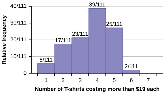
The percentage of people who own at most three T-shirts costing more than $19 each is approximately ________.
a. 21
b. 59
c. 41
d. cannot be determined
Answer
2-85 §2.2 source ↗
Use the following information to answer the next two exercises: Suppose 111 people who shopped in a special T-shirt store were asked the number of T-shirts they own costing more than $19 each.
Following are the 2010 obesity rates by U.S. states and Washington, DC.
Construct a bar graph of obesity rates of your state and the four states closest to your state. Hint—Label the x-axis with the states.
| State | Percent (%) | State | Percent (%) | State | Percent (%) |
|---|---|---|---|---|---|
| Alabama | 32.2 | Kentucky | 31.3 | North Dakota | 27.2 |
| Alaska | 24.5 | Louisiana | 31.0 | Ohio | 29.2 |
| Arizona | 24.3 | Maine | 26.8 | Oklahoma | 30.4 |
| Arkansas | 30.1 | Maryland | 27.1 | Oregon | 26.8 |
| California | 24.0 | Massachusetts | 23.0 | Pennsylvania | 28.6 |
| Colorado | 21.0 | Michigan | 30.9 | Rhode Island | 25.5 |
| Connecticut | 22.5 | Minnesota | 24.8 | South Carolina | 31.5 |
| Delaware | 28.0 | Mississippi | 34.0 | South Dakota | 27.3 |
| Washington, DC | 22.2 | Missouri | 30.5 | Tennessee | 30.8 |
| Florida | 26.6 | Montana | 23.0 | Texas | 31.0 |
| Georgia | 29.6 | Nebraska | 26.9 | Utah | 22.5 |
| Hawaii | 22.7 | Nevada | 22.4 | Vermont | 23.2 |
| Idaho | 26.5 | New Hampshire | 25.0 | Virginia | 26.0 |
| Illinois | 28.2 | New Jersey | 23.8 | Washington | 25.5 |
| Indiana | 29.6 | New Mexico | 25.1 | West Virginia | 32.5 |
| Iowa | 28.4 | New York | 23.9 | Wisconsin | 26.3 |
| Kansas | 29.4 | North Carolina | 27.8 | Wyoming | 25.1 |
Answer
2-87 §2.3 source ↗
Six hundred adult Americans were asked by telephone poll, "What do you think constitutes a middle-class income?" The results are in Table 2.72. Also, include the left endpoint but not the right endpoint.
a. What percentage of the survey answered "not sure"?
b. What percentage think that middle class is from $25,000 to $50,000?
c. Construct a histogram of the data.
i. Should all bars have the same width, based on the data? Why or why not?
ii. How should the < 20,000 and the 100,000+ intervals be handled? Why?
d. Find the 40th and 80th percentiles.
e. Construct a bar graph of the data.
| Salary ($) | Relative Frequency |
|---|---|
| < 20,000 | .02 |
| 20,000–25,000 | .09 |
| 25,000–30,000 | .19 |
| 30,000–40,000 | .26 |
| 40,000–50,000 | .18 |
| 50,000–75,000 | .17 |
| 75,000–99,999 | .02 |
| 100,000+ | .01 |
Answer
a. 1 – (.02+.09+.19+.26+.18+.17+.02+.01) = .06
b. .19+.26+.18 = .63
c. Check student’s solution.
d.
40th percentile will fall between 30,000 and 40,000
80th percentile will fall between 50,000 and 75,000
e. Check student’s solution.
2-89 §2.3 source ↗
The following box plot shows the ages of the U.S. population for 1990, the latest available year:
a. Are there fewer or more children (age 17 and under) than senior citizens (age 65 and over)? How do you know?
b. 12.6 percent are age 65 and over. Approximately what percentage of the population are working-age adults (above age 17 to age 65)?
Answer
a. more children; the left whisker shows that 25 percent of the population are children 17 and younger; the right whisker shows that 25 percent of the population are adults 50 and older, so adults 65 and over represent less than 25 percent
b. 62.4 percent
2-91 §2.4 source ↗
Given the following box plot, answer the questions.
a. Think of an example (in words) where the data might fit into the above box plot. In two to five sentences, write down the example.
b. What does it mean to have the first and second quartiles so close together, while the second to third quartiles are far apart?
Answer
a. Answers will vary. Possible answer: State University conducted a survey to see how involved its students are in community service. The box plot shows the number of community service hours logged by participants over the past year.
b. Because the first and second quartiles are close, the data in this quarter is very similar. There is not much variation in the values. The data in the third quarter is much more variable, or spread out. This is clear because the second quartile is so far away from the third quartile.
2-93 §2.4 source ↗
A survey was conducted of 130 purchasers of new black sports cars, 130 purchasers of new red sports cars, and 130 purchasers of new white sports cars. In it, people were asked the age they were when they purchased their car. The following box plots display the results:
a. In complete sentences, describe what the shape of each box plot implies about the distribution of the data collected for that car series.
b. Which group is most likely to have an outlier? Explain how you determined that.
c. Compare the three box plots. What do they imply about the age of purchasing a sports car from the series when compared to each other?
d. Look at the red sports cars. Which quarter has the smallest spread of data? What is the spread?
e. Look at the red sports cars. Which quarter has the largest spread of data? What is the spread?
f. Look at the red sports cars. Estimate the interquartile range (IQR).
g. Look at the red sports cars. Are there more data in the interval 31–38 or in the interval 45–55? How do you know this?
h. Look at the red sports cars. Which interval has the fewest data in it? How do you know this?
i. 31–35
ii. 38–41
iii. 41–64
Answer
a. Each box plot is spread out more in the greater values. Each plot is skewed to the right, so the ages of the top 50 percent of buyers are more variable than the ages of the lower 50 percent.
b. The black sports car is most likely to have an outlier. It has the longest whisker.
c. Comparing the median ages, younger people tend to buy the black sports car, while older people tend to buy the white sports car. However, this is not a rule, because there is so much variability in each data set.
d. The second quarter has the smallest spread. There seems to be only a three-year difference between the first quartile and the median.
e. The third quarter has the largest spread. There seems to be approximately a 14-year difference between the median and the third quartile.
f. IQR ~ 17 years
g. There is not enough information to tell. Each interval lies within a quarter, so we cannot tell exactly where the data in that quarter is are concentrated.
h. The interval from 31 to 35 years has the fewest data values. Twenty-five percent of the values fall in the interval 38 to 41, and 25 percent fall between 41 and 64. Since 25 percent of values fall between 31 and 38, we know that fewer than 25 percent fall between 31 and 35.
2-96 §2.5 source ↗
| Percentage of Children with the Condition | Number of Countries |
|---|---|
| 16–21.45 | 23 |
| 21.45–26.9 | 4 |
| 26.9–32.35 | 9 |
| 32.35–37.8 | 7 |
| 37.8–43.25 | 6 |
| 43.25–48.7 | 1 |
Answer
2-98 §2.7 source ↗
Use the following information to answer the next nine exercises: The population parameters below describe the full-time equivalent number of students (FTES) each year at Lake Tahoe Community College from 1976–1977 through 2004–2005.
A sample of 11 years is taken. About how many are expected to have an FTES of 1,014 or above? Explain how you determined your answer.
Answer
2-100 §2.7 source ↗
Use the following information to answer the next nine exercises: The population parameters below describe the full-time equivalent number of students (FTES) each year at Lake Tahoe Community College from 1976–1977 through 2004–2005.
The population standard deviation = ______.
Answer
2-102 §2.7 source ↗
Use the following information to answer the next nine exercises: The population parameters below describe the full-time equivalent number of students (FTES) each year at Lake Tahoe Community College from 1976–1977 through 2004–2005.
What is the IQR? What does the IQR represent?
Answer
2-104 §2.7 source ↗
Use the following information to answer the next nine exercises: The population parameters below describe the full-time equivalent number of students (FTES) each year at Lake Tahoe Community College from 1976–1977 through 2004–2005.
Calculate the mean, median, standard deviation, the first quartile, the third quartile, and the IQR. Round to one decimal place.
Answer
• mean = 1,809.3
• median = 1,812.5
• standard deviation = 151.2
• first quartile = 1,690
• third quartile = 1,935
• IQR = 245
2-106 §2.7 source ↗
Use the following information to answer the next nine exercises: The population parameters below describe the full-time equivalent number of students (FTES) each year at Lake Tahoe Community College from 1976–1977 through 2004–2005.
Compare the IQR for the FTES for 1976–1977 through 2004–2005 with the IQR for the FTES for 2005-2006 through 2010–2011. Why do you suppose the IQRs are so different?
Answer
2-108 §2.7 source ↗
Use the following information to answer the next nine exercises: The population parameters below describe the full-time equivalent number of students (FTES) each year at Lake Tahoe Community College from 1976–1977 through 2004–2005.
A music school has budgeted to purchase three musical instruments. The school plans to purchase a piano costing $3,000, a guitar costing $550, and a drum set costing $600. The mean cost for a piano is $4,000 with a standard deviation of $2,500. The mean cost for a guitar is $500 with a standard deviation of $200. The mean cost for drums is $700 with a standard deviation of $100. Which cost is the lowest when compared to other instruments of the same type? Which cost is the highest when compared to other instruments of the same type? Justify your answer.
Answer
2-110 §2.7 source ↗
Use the following information to answer the next nine exercises: The population parameters below describe the full-time equivalent number of students (FTES) each year at Lake Tahoe Community College from 1976–1977 through 2004–2005.
Scientists are studying a particular disease. They found that countries that have the highest rates of people who have ever been diagnosed with this disease range from 11.4 percent to 74.6 percent.
What is the best estimate of the average percentage of people with the disease for these countries? What is the standard deviation for the listed rates? The United States has an average disease rate of 33.9 percent. Is this rate above average or below? How unusual is the U.S. obesity rate compared to the average rate? Explain.
| Percentage of Population with Disease | Number of Countries |
|---|---|
| 11.4–20.45 | 29 |
| 20.45–29.45 | 13 |
| 29.45–38.45 | 4 |
| 38.45–47.45 | 0 |
| 47.45–56.45 | 2 |
| 56.45–65.45 | 1 |
| 65.45–74.45 | 0 |
| 74.45–83.45 | 1 |
Answer
•
• Using the TI 83/84, we obtain a standard deviation of:
• The obesity rate of the United States is 10.58 percent higher than the average obesity rate.
• Since the standard deviation is 12.95, we see that 23.32 + 12.95 = 36.27 is the disease percentage that is one standard deviation from the mean. The U.S. disease rate is slightly less than one standard deviation from the mean. Therefore, we can assume that the United States, although 34 percent have the disease, does not have an unusually high percentage of people with the disease.
2-112 §2.BIT source ↗
Santa Clara County, California, has approximately 27,873 Japanese Americans. Table 2.80 shows their ages by group and each age-group's percentage of the Japanese American community.
a. Construct a histogram of the Japanese American community in Santa Clara County. The bars will not be the same width for this example. Why not? What impact does this have on the reliability of the graph?
b. What percentage of the community is under age 35?
c. Which box plot most resembles the information above?
| Age-Group | Percentage of Community |
|---|---|
| 0–17 | 18.9 |
| 18–24 | 8.0 |
| 25–34 | 22.8 |
| 35–44 | 15.0 |
| 45–54 | 13.1 |
| 55–64 | 11.9 |
| 65+ | 10.3 |
Answer
a. For graph, check student's solution.
b. 49.7 percent of the community is under the age of 35
c. Based on the information in the table, graph (a) most closely represents the data.
2-114 §2.BIT source ↗
Use the following information to answer the next three exercises: We are interested in the number of years students in a particular elementary statistics class have lived in California. The information in the following table is from the entire section.
What is the IQR?
a. 8
b. 11
c. 15
d. 35
| Number of Years | Frequency | Number of Years | Frequency |
|---|---|---|---|
| 7 | 1 | 22 | 1 |
| 14 | 3 | 23 | 1 |
| 15 | 1 | 26 | 1 |
| 18 | 1 | 40 | 2 |
| 19 | 4 | 42 | 2 |
| 20 | 3 | ||
| Total = 20 |
Answer
2-116 §2.BIT source ↗
Use the following information to answer the next three exercises: We are interested in the number of years students in a particular elementary statistics class have lived in California. The information in the following table is from the entire section.
Is this a sample or the entire population?
a. sample
b. entire population
c. neither
| Number of Years | Frequency | Number of Years | Frequency |
|---|---|---|---|
| 7 | 1 | 22 | 1 |
| 14 | 3 | 23 | 1 |
| 15 | 1 | 26 | 1 |
| 18 | 1 | 40 | 2 |
| 19 | 4 | 42 | 2 |
| 20 | 3 | ||
| Total = 20 |
Answer
2-117 §2.BIT source ↗
Twenty-five randomly selected students were asked the number of movies they watched the previous week. The results are as follows:
a. Find the sample mean .
b. Find the approximate sample standard deviation, s.
| Number of Movies | Frequency |
|---|---|
| 0 | 5 |
| 1 | 9 |
| 2 | 6 |
| 3 | 4 |
| 4 | 1 |
Answer
a. 1.48
b. 1.12
2-119 §2.BIT source ↗
Following are the published weights (in pounds) of all of the football team members of the San Francisco 49ers from a previous year:
177, 205, 210, 210, 232, 205, 185, 185, 178, 210, 206, 212, 184, 174, 185, 242, 188, 212, 215, 247, 241, 223, 220, 260, 245, 259, 278, 270, 280, 295, 275, 285, 290, 272, 273, 280, 285, 286, 200, 215, 185, 230, 250, 241, 190, 260, 250, 302, 265, 290, 276, 228, 265
a. Organize the data from smallest to largest value.
b. Find the median.
c. Find the first quartile.
d. Find the third quartile.
e. Construct a box plot of the data.
f. The middle 50 percent of the weights are from ________ to ________.
g. If our population were all professional football players, would the above data be a sample of weights or the population of weights? Why?
h. If our population included every team member who ever played for a California-based football team, would the above data be a sample of weights or the population of weights? Why?
i. Assume the population was a California-based football team. Find
i. the population mean, μ,
ii. the population standard deviation, σ, and
iii. the weight that is two standard deviations below the mean.
iv. In addition, when the team's most famous quarterback, played football, he weighed 205 pounds. Also find how many standard deviations above or below the mean was he?
j. That same year, the mean weight for a player from a Texas football team was 240.08 pounds with a standard deviation of 44.38 pounds. One player weighed in at 209 pounds. With respect to his team, who was lighter, the California quarterback or the Texas player? How did you determine your answer?
Answer
a. 174, 177, 178, 184, 185, 185, 185, 185, 188, 190, 200, 205, 205, 206, 210, 210, 210, 212, 212, 215, 215, 220, 223, 228, 230, 232, 241, 241, 242, 245, 247, 250, 250, 259, 260, 260, 265, 265, 270, 272, 273, 275, 276, 278, 280, 280, 285, 285, 286, 290, 290, 295, 302
b. 241
c. 205.5
d. 272.5
e. 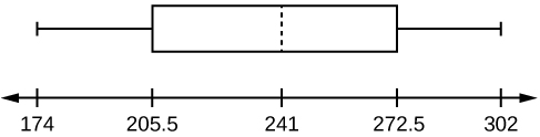
f. 205.5, 272.5
g. sample
h. population
i.
i. 236.34
ii. 37.50
iii. 161.34
iv. .84 standard deviations below the mean
j. young
2-121 §2.BIT source ↗
Refer to Figure 2.52 to determine which of the following are true and which are false. Explain your solution to each part in complete sentences.
a. The medians for all three graphs are the same.
b. We cannot determine if any of the means for the three graphs are different.
c. The standard deviation for Graph b is larger than the standard deviation for Graph a.
d. We cannot determine if any of the third quartiles for the three graphs are different.
Answer
a. true
b. true
c. true
d. false
2-123 §2.BIT source ↗
A survey of enrollment at 35 community colleges across the United States yielded the following figures:
6,414; 1,550; 2,109; 9,350; 21,828; 4,300; 5,944; 5,722; 2,825; 2,044; 5,481; 5,200; 5,853; 2,750; 10,012; 6,357; 27,000; 9,414; 7,681; 3,200; 17,500; 9,200; 7,380; 18,314; 6,557; 13,713; 17,768; 7,493; 2,771; 2,861; 1,263; 7,285; 28,165; 5,080; 11,622
a. Organize the data into a chart with five intervals of equal width. Label the two columns Enrollment and Frequency.
b. Construct a histogram of the data.
c. If you were to build a new community college, which piece of information would be more valuable: the mode or the mean?
d. Calculate the sample mean.
e. Calculate the sample standard deviation.
f. A school with an enrollment of 8,000 would be how many standard deviations away from the mean?
Answer
a.
| Enrollment | Frequency |
|---|---|
| 1,000–5,000 | 10 |
| 5,000–10,000 | 16 |
| 10,000–15,000 | 3 |
| 15,000–20,000 | 3 |
| 20,000–25,000 | 1 |
| 25,000–30,000 | 2 |
b. Check student’s solution.
c. mode
d. 8,628.74
e. 6,943.88
f. –0.09
| Enrollment | Frequency |
|---|---|
| 1,000–5,000 | 10 |
| 5,000–10,000 | 16 |
| 10,000–15,000 | 3 |
| 15,000–20,000 | 3 |
| 20,000–25,000 | 1 |
| 25,000–30,000 | 2 |
2-125 §2.BIT source ↗
Use the following information to answer the next two exercises. X = the number of days per week that 100 clients use a particular exercise facility.
The number that is 1.5 standard deviations below the mean is approximately ________.
a. 0.7
b. 4.8
c. –2.8
d. cannot be determined
| X | Frequency |
|---|---|
| 0 | 3 |
| 1 | 12 |
| 2 | 33 |
| 3 | 28 |
| 4 | 11 |
| 5 | 9 |
| 6 | 4 |
Answer
Loading chapter 3…
Problems and answers are adapted from Statistics by Barbara Illowsky and Susan Dean, attributed to the Texas Education Agency (TEA) and published by OpenStax, and are used under the CC BY 4.0 licence. Access for free at https://openstax.org/books/statistics/pages/1-introduction. The original material is available at https://www.texasgateway.org/book/tea-statistics. Changes were made to the original material, including updates to art, structure, and other content updates. Art is credited in its own caption wherever the book credits it. This adaptation is neither affiliated with nor endorsed by OpenStax, Rice University or the Texas Education Agency (TEA).