Every problem in the chapter beside the book’s answer, a chapter at a time as you scroll.
Chapter 2: First-order equations
43 problems · 4 figuresExercise 1.1.101 §1.1 source ↗
Solve and .
Answer
Exercise 1.1.102 §1.1 source ↗
Solve , .
Answer
Exercise 1.1.103 §1.1 source ↗
Solve , .
Answer
Exercise 1.1.104 §1.1 source ↗
Sid is in a car traveling at speed miles per hour away from Las Vegas, where is in hours. At , Sid is 10 miles away from Vegas. How far from Vegas is Sid 2 hours later?
Answer
170
Exercise 1.1.105 §1.1 source ↗
Solve , , where is a positive integer. Hint: You have to consider different cases.
Answer
If , then . If , then .
Exercise 1.1.106 §1.1 source ↗
The rate of change of the volume of a snowball that is melting is proportional to the surface area of the snowball. Suppose the snowball is perfectly spherical. The volume (in centimeters cubed) of a ball of radius centimeters is . The surface area is . Set up the differential equation for how the radius is changing. Then, suppose that at time minutes, the radius is 10 centimeters. After 5 minutes, the radius is 8 centimeters. At what time will the snowball be completely melted?
Answer
The equation is for some constant . The snowball will be completely melted in 25 minutes from time .
Exercise 1.1.107 §1.1 source ↗
Find the general solution to . How many distinct constants do you need?
Answer
, so 4 constants.
Exercise 1.2.101 §1.2 source ↗
Sketch the slope field of . Can you visually find the solution that satisfies ?
Answer (2 parts)
is a solution such that .
Exercise 1.2.102 §1.2 source ↗
Is it possible to solve for ? Is the solution unique?
Answer
Yes a solution exists. The equation is where . The function is continuous and , which is also continuous near . So a solution exists and is unique. (In fact, is the solution.)
Exercise 1.2.103 §1.2 source ↗
Is it possible to solve for ?
Answer
No, the equation is not defined at .
Exercise 1.2.104 §1.2 source ↗
Match equations , , to slope fields. Justify.
a)
b)
c)
Answer
a) , b) , c) . Justification left to reader.
Exercise 1.2.105 §1.2 source ↗
(tricky) Suppose
Does , have a continuously differentiable solution? Does Picard apply? Why, or why not?
Answer
Picard does not apply as is not continuous at . The equation does not have a continuously differentiable solution. Suppose it did. Notice that . By the first derivative test, for small positive . But then for those , we have . It is not possible for to be continuous, and for arbitrarily small positive .
Exercise 1.2.106 §1.2 source ↗
Consider an equation of the form for some continuous function , and an initial condition . Does a solution exist for all ? Why or why not?
Answer
The solution is , and this does indeed exist for every .
Exercise 1.3.101 §1.3 source ↗
Solve .
Answer
Exercise 1.3.102 §1.3 source ↗
Solve , .
Answer
Exercise 1.3.103 §1.3 source ↗
Find an implicit solution for , .
Answer
Exercise 1.3.104 §1.3 source ↗
Find an explicit solution to , .
Answer
Exercise 1.3.105 §1.3 source ↗
Find an implicit solution to .
Answer
Exercise 1.3.106 §1.3 source ↗
Take Example 1.3.3 with the same numbers: 89 degrees at , 85 degrees at , and ambient temperature of 22 degrees. Suppose these temperatures were measured with a precision of degrees. Given this imprecision, the time it takes the coffee to cool to (exactly) 60 degrees is also only known in a certain range. Find this range. Hint: Think about what kind of error makes the cooling time longer and what shorter.
Bob made a cup of coffee, and Bob likes to drink coffee only once it reaches 60 degrees Celsius and will not burn him. Initially, right after it was poured in the cup, Bob measured the temperature and the coffee was 89 degrees Celsius. One minute later, Bob measured the coffee again and it had 85 degrees. The temperature of the room (the ambient temperature) is 22 degrees. When should Bob start drinking?
Let be the temperature of the coffee in degrees Celsius, let be the ambient (room) temperature, also in degrees Celsius, and let denote the time in minutes, with denoting the time when Bob made the coffee. Newton’s law of cooling states that the rate at which the temperature of the coffee is changing is proportional to the difference between the ambient temperature and the temperature of the coffee. That is,
for some positive constant . For our setup , , . Let and denote arbitrary constants, and notice that since the coffee is clearly warmer than the room. We separate variables and integrate.
That is, . We plug in the first condition: , and hence . So . The second condition says . Solving for , we get . We solve for the time that gives a temperature of 60 degrees. Namely, we solve
to get minutes. So Bob can begin to drink the coffee at just over 9 minutes from the time Bob made it. That is probably about the amount of time it took us to calculate how long it would take. See Figure 1.7.
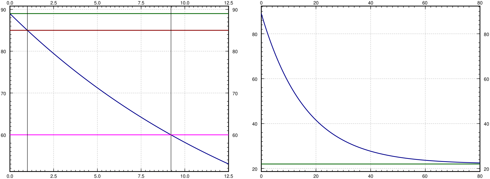
Graphs of the coffee temperature function . On the left, horizontal lines are drawn at temperatures 60, 85, and 89. Vertical lines are drawn at and . Notice that the temperature of the coffee hits 85 at , and 60 at . On the right, the graph is over a longer period of time, with a horizontal line at the ambient temperature 22.
Graphs of the coffee temperature function . On the left, horizontal lines are drawn at temperatures 60, 85, and 89. Vertical lines are drawn at and . Notice that the temperature of the coffee hits 85 at , and 60 at . On the right, the graph is over a longer period of time, with a horizontal line at the ambient temperature 22.
Answer
The range is approximately 7.45 to 12.15 minutes.
Exercise 1.3.107 §1.3 source ↗
A population of rabbits on an island is modeled by , where the independent variable is time in months. At time , there are 40 rabbits on the island.
a) Find the solution to the equation with the initial condition.
b) How many rabbits are on the island in 1 month, 5 months, 10 months, 15 months (round to the nearest integer)?
Answer
a) . b) 102 rabbits after one month, 861 after 5 months, 999 after 10 months, 1000 after 15 months.
Exercise 1.4.101 §1.4 source ↗
Solve .
Answer
Exercise 1.4.102 §1.4 source ↗
Solve , .
Answer
Exercise 1.4.103 §1.4 source ↗
Suppose a water tank is being pumped out at . The water tank starts at of clean water. Water with a toxic substance is flowing into the tank at , with concentration at time . When the tank is half empty, how many grams of toxic substance are in the tank (assuming perfect mixing)?
Answer
grams
Exercise 1.4.104 §1.4 source ↗
There are bacteria on a plate and a toxic substance is being added that slows down the rate of growth of the bacteria. That is, suppose that . If , find the population at .
Answer
Exercise 1.4.105 §1.4 source ↗
A cylindrical water tank has water flowing in at cubic meters per second. Let be the area of the cross section of the tank in square meters. Suppose water is flowing out from the bottom of the tank at a rate proportional to the height of the water level. Set up the differential equation for , the height of the water, introducing and naming constants that you need. You should also give the units for your constants.
Answer
, where is a constant with units .
Exercise 1.5.101 §1.5 source ↗
Solve , .
Answer
Exercise 1.5.102 §1.5 source ↗
Solve , .
Answer
Exercise 1.5.103 §1.5 source ↗
Solve , .
Answer
Exercise 1.5.104 §1.5 source ↗
Solve .
Answer
Exercise 1.6.101 §1.6 source ↗
Let .
a) Sketch the phase diagram and find critical points.
b) Classify the critical points.
c) If , then find .
Answer
a) 0, 1, 2 are critical points. b) is unstable (semistable), is stable, and is unstable. c) 1
Exercise 1.6.102 §1.6 source ↗
Let .
a) Find and classify all critical points.
b) Find given any initial condition.
Answer
a) There are no critical points. b)
Exercise 1.6.103 §1.6 source ↗
Assume that a population of fish in a lake satisfies . Now suppose that fish are continually added at fish per unit of time.
a) Find the differential equation for .
b) What is the new limiting population?
Answer
a) b)
Exercise 1.6.104 §1.6 source ↗
Suppose for two numbers .
a) Find the critical points, and classify them.
For b), c), d), find based on the phase diagram.
a) ,
b) ,
c) .
Answer
a) is a stable critical point, is an unstable one. b) , c) , d) or DNE.
Exercise 1.7.101 §1.7 source ↗
Let , and . Approximate using Euler’s method with step sizes 1, 0.5, 0.25. Use a calculator and compute up to 4 decimal digits.
Answer
Approximately: 1.0000, 1.2397, 1.3829
Exercise 1.7.102 §1.7 source ↗
Let , and .
a) Approximate using Euler’s method with step sizes 4, 2, and 1.
b) Solve exactly, and compute the errors.
c) Compute the factor by which the errors changed.
Answer
a) 0, 8, 12 b) , so errors are: 16, 8, 4. c) Factors are 0.5 and 0.5.
Exercise 1.7.103 §1.7 source ↗
Let , and .
a) Approximate using Euler’s method with step sizes 4, 2, and 1.
b) Guess an exact solution based on part a) and compute the errors.
Answer
a) 0, 0, 0 b) is a solution so errors are: 0, 0, 0.
Exercise 1.7.104 §1.7 source ↗
Consider , .
a) Approximate using the improved Euler’s method (see above) with step sizes and .
b) Approximate using Euler’s method with and .
c) Solve exactly, find the exact value of .
d) Compute the errors, and the factors by which the errors changed.
Answer
a) Improved Euler: for , for , b) Standard Euler: for , for , c) , so is approximately . d) Approximate errors for improved Euler: for and for . For standard Euler: for and for . Factor is approximately for improved Euler and for standard Euler.
Exercise 1.8.101 §1.8 source ↗
Solve the following exact equations, implicit general solutions will suffice:
a)
b)
c)
d)
Answer
a) b) c) d)
Exercise 1.8.102 §1.8 source ↗
Find the integrating factor for the following equations making them into exact equations:
a)
b)
c)
d)
Answer
a) Integrating factor is , equation becomes . b) Integrating factor is , equation becomes . c) Integrating factor is , equation becomes . d) Integrating factor is , equation becomes .
Exercise 1.8.103 §1.8 source ↗
a) Show that every separable equation can be written as an exact equation, and verify that it is indeed exact.
b) Rewrite as an exact equation, solve it, and verify that the solution is the same as it was in Example 1.3.1.
Take the equation
Note that is a solution. We will remember that fact and assume from now on, so that we can divide by . Write the equation as or . Then
We compute the antiderivatives to get
or
where is some constant. Because is also a solution and because of the absolute value, we can write:
for any number (including zero or negative).
We check:
Yay!
Answer
a) The equation is , and this is exact because , , so . b) , leads to potential function , solving leads to the same solution as the example.
Exercise 1.9.101 §1.9 source ↗
Solve
a) , ,
b) , .
Answer
a) b)
Exercise 1.9.102 §1.9 source ↗
Solve , .
Answer
Exercise 1.9.103 §1.9 source ↗
Solve , .
Answer
Loading chapter 3…
Exercises and answers are adapted from Notes on Diffy Qs: Differential Equations for Engineers by Jiří Lebl, which is free to read and download, and are used under the CC BY-NC-SA 4.0 licence. They are taken from the book’s LaTeX source and set for the web, so they may differ slightly from the printed page. This adaptation is released under the same licence and is neither affiliated with nor endorsed by Lebl or Jiří Lebl.