Every problem in the chapter beside the book’s answer, a chapter at a time as you scroll.
Chapter 15: Poverty and Economic Inequality
13 problems · 5 figures15-1 §15.1 source ↗
Describe how each of these changes is likely to affect poverty and inequality:
a. Incomes rise for low-income and high-income workers, but rise more for the high-income earners.
b. Incomes fall for low-income and high-income workers, but fall more for high-income earners.
Answer
a. Poverty falls, inequality rises.
b. Poverty rises, inequality falls.
15-2 §15.2 source ↗
| Amount Worked (hours) | Total Earnings | Government Support | Total Income |
|---|---|---|---|
| 0 | 0 | $18,000 | $18,000 |
| 500 | $4,000 | $16,000 | $20,000 |
| 1,000 | $8,000 | $14,000 | $22,000 |
| 1,500 | $12,000 | $12,000 | $24,000 |
| 2,000 | $16,000 | $10,000 | $26,000 |
| 2,500 | $20,000 | $8,000 | $28,000 |
Answer
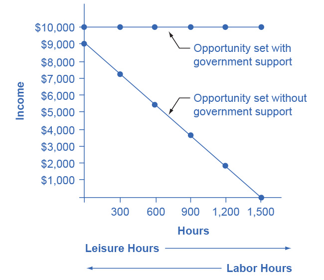
Jonathon’s options for working and total income are shown in the following table. His labor-leisure diagram is shown in the figure following the table.
| Number of Work Hours | Earnings from Work | Government Benefits | Total Income |
|---|---|---|---|
| 1,500 | $9,000 | $1,000 | $10,000 |
| 1,200 | $7,200 | $2,800 | $10,000 |
| 900 | $5,400 | $4,600 | $10,000 |
| 600 | $3,600 | $6,400 | $10,000 |
| 300 | $1,800 | $8,200 | $10,000 |
| 0 | $0 | $10,000 | $10,000 |
15-3 §15.2 source ↗
Answer
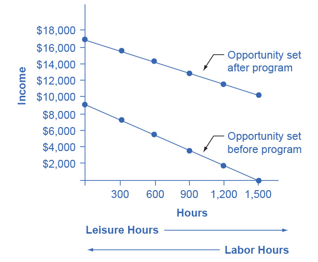
The following table shows a policy where only 30 cents in government support is pulled right back for every $1 of income earned. Jonathon’s labor-leisure diagram is shown in the figure following the table. “Opportunity set after program” extends from (0, $16,300) to (1,500, $10,000). “Opportunity set before program” slopes downward from (0, $9,000) to (1,500, $0).
| Number of Work Hours | Earnings from Work | Government Benefits | Total Income |
|---|---|---|---|
| 1,500 | $9,000 | $7,300 | $16,300 |
| 1,200 | $7,200 | $7,840 | $15,040 |
| 900 | $5,400 | $8,380 | $13,780 |
| 600 | $3,600 | $8,920 | $12,520 |
| 300 | $1,800 | $9,460 | $22,260 |
| 0 | $0 | $10,000 | $10,000 |
15-4 §15.3 source ↗
Answer
15-5 §15.3 source ↗
Answer
15-6 §15.4 source ↗
Answer
A useful first step is to rank the households by income, from lowest to highest. Then, since there are 10 households total, the bottom quintile will be the bottom two households, the second quintile will be the third and fourth households, and so on up to the top quintile. The quintiles and percentage of total income for the data provided are shown in the following table. Comparing this distribution to the U.S. income distribution for 2005, the top quintile in the example has a smaller share of total income than in the U.S. distribution and the bottom quintile has a larger share. This pattern usually means that the income distribution in the example is more equal than the U.S. distribution.
| Income | Quintile | % of Total Income |
|---|---|---|
| $10,000 | Total first quintile income: $22,000 | 6.0% |
| $12,000 | ||
| $16,000 | Total second quintile income: $34,000 | 9.2% |
| $18,000 | ||
| $24,000 | Total third quintile income: $48,000 | 13.0% |
| $24,000 | ||
| $36,000 | Total fourth quintile income: $86,000 | 23.2% |
| $50,000 | ||
| $80,000 | Total top quintile income: $180,000 | 48.6% |
| $100,000 | ||
| $370,000 | Total Income |
15-7 §15.4 source ↗
| Share of Income | 1979 | 1991 |
|---|---|---|
| Top quintile | 39.7% | 42.9% |
| Fourth quintile | 24.8% | 22.7% |
| Middle quintile | 17.0% | 16.3% |
| Second quintile | 11.5% | 11.5% |
| Bottom quintile | 7.0% | 6.6% |
Answer
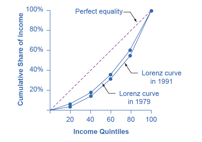
Just from glancing at the quintile information, it is fairly obvious that income inequality increased in the United Kingdom over this time: The top quintile is getting a lot more, and the lowest quintile is getting a bit less. Converting this information into a Lorenz curve, however, is a little trickier, because the Lorenz curve graphs the cumulative distribution, not the amount received by individual quintiles. Thus, as explained in the text, you have to add up the individual quintile data to convert the data to this form. The following table shows the actual calculations for the share of income in 1979 versus 1991. The figure following the table shows the perfect equality line and the Lorenz curves for 1979 and 1991. As shown, the income distribution in 1979 was closer to the perfect equality line than the income distribution in 1991—that is, the United Kingdom income distribution became more unequal over time.
| Share of income received | 1979 | 1991 |
|---|---|---|
| Bottom 20% | 7.0% | 6.6% |
| Bottom 40% | 18.5% | 18.1% |
| Bottom 60% | 35.5% | 34.4% |
| Bottom 80% | 60.3% | 57.1% |
| All 100% | 100.0% | 100.0% |
15-8 §15.4 source ↗
Answer
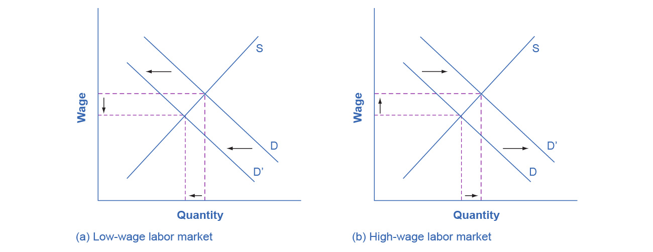
In the market for low-wage labor, information technology shifts the demand for low-wage labor to the left. One reason is that technology can often substitute for low-wage labor in certain kinds of telephone or bookkeeping jobs. In addition, information technology makes it easier for companies to manage connections with low-wage workers in other countries, thus reducing the demand for low-wage workers in the United States. In the market for high-wage labor, information technology shifts the demand for high-wage labor to the right. By using the new information and communications technologies, high-wage labor can become more productive and can oversee more tasks than before. The following figure illustrates these two labor markets. The combination of lower wages for low-wage labor and higher wages for high-wage labor means greater inequality.
15-9 §15.4 source ↗
Answer
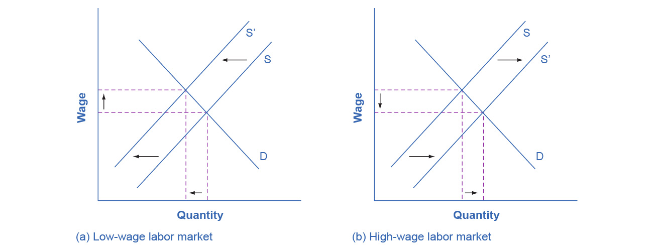
In the market for low-wage labor, a skills program will shift supply to the left, which will tend to drive up wages for the remaining low-skill workers. In the market for high-wage labor, a skills program will shift supply to the right (because after the training program there are now more high-skilled workers at every wage), which will tend to drive down wages for high-skill workers. The combination of these two programs will result in a lesser degree of inequality. The following figure illustrates these two labor markets. In the market for high-wage labor, a skills program will shift supply to the right, which will tend to drive down wages for high-skill workers.
15-10 §15.5 source ↗
Answer
15-11 §15.5 source ↗
Answer
15-12 §15.5 source ↗
Answer
15-13 §15.5 source ↗
Answer
Loading chapter 16…
Problems and answers are adapted from Principles of Microeconomics 3e by Steven A. Greenlaw, David Shapiro and Daniel MacDonald, OpenStax, and are used under the CC BY-NC-SA 4.0 licence. Access for free at https://openstax.org/books/principles-microeconomics-3e/pages/1-introduction. Illustrations: Copyright Rice University, OpenStax, under CC BY-NC-SA 4.0 license. This adaptation is released under the same licence, is non-commercial, and is neither affiliated with nor endorsed by OpenStax or Rice University.