Chapter 5: Important Distributions and DensitiesContent check — Probability (Grinstead and Snell), Chapter 5: Important Distributions and Densities

A number $U$ is chosen at random in the interval $[\mathrm{0,1}]$⁠. Find the probability that

(a) $R=U^2<1/4$⁠.

(b) $S=U(1-U)<1/4$⁠.

(c) $T=U/(1-U)<1/4$⁠.

A point $P$ in the unit square has coordinates $X$ and $Y$ chosen at random in the interval $[\mathrm{0,1}]$⁠. Let $D$ be the distance from $P$ to the nearest edge of the square, and $E$ the distance to the nearest corner. What is the probability that

(a) $D<1/4$⁠?

(b) $E<1/4$⁠?

Let $X$ be a random variable with cumulative distribution function $F_X$⁠, and let $Y=X+b$⁠, $Z=aX$⁠, and $W=aX+b$⁠, where $a$ and $b$ are any constants. Find the cumulative distribution functions $F_Y$⁠, $F_Z$⁠, and $F_W$⁠. Hint: The cases $a>0$⁠, $a=0$⁠, and $a<0$ require different arguments.

Let $X$ be a random variable with cumulative distribution function $F$⁠. The median of $X$ is the value $m$ for which $F(m)=1/2$⁠. Then $X<m$ with probability 1/2 and $X>m$ with probability 1/2. Find $m$ if $X$ is

(a) uniformly distributed over the interval $[a,b]$⁠.

(b) normally distributed with parameters $\mu$ and $\sigma$⁠.

(c) exponentially distributed with parameter $\lambda$⁠.

Grading on the curve.

(Queues) Suppose that customers arrive at random times at a service station with one server, and suppose that each customer is served immediately if no one is ahead of him, but must wait his turn in line otherwise. How long should each customer expect to wait? (We define the waiting time of a customer to be the length of time between the time that he arrives and the time that he begins to be served.)

Let us assume that the interarrival times between successive customers are given by random variables $X_1$⁠, $X_2$⁠, …, $X_n$ that are mutually independent and identically distributed with an exponential cumulative distribution function given by $$F_X(t)=1-e^{-\lambda t}.$$ Let us assume, too, that the service times for successive customers are given by random variables $Y_1$⁠, $Y_2$⁠, …, $Y_n$ that again are mutually independent and identically distributed with another exponential cumulative distribution function given by $$F_Y(t)=1-e^{-\mu t}.$$

The parameters $\lambda$ and $\mu$ represent, respectively, the reciprocals of the average time between arrivals of customers and the average service time of the customers. Thus, for example, the larger the value of $\lambda$⁠, the smaller the average time between arrivals of customers. We can guess that the length of time a customer will spend in the queue depends on the relative sizes of the average interarrival time and the average service time.

It is easy to verify this conjecture by simulation. The program Queue simulates this queueing process. Let $N(t)$ be the number of customers in the queue at time $t$⁠. Then we plot $N(t)$ as a function of $t$ for different choices of the parameters $\lambda$ and $\mu$ (see Figure 5.7).

Figure 5.7: Queue sizes.

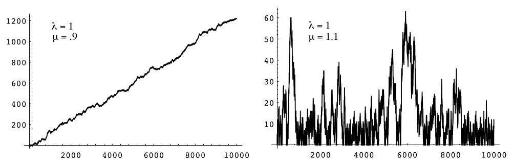
We note that when $\lambda <\mu$⁠, then $1/\lambda >1/\mu$⁠, so the average interarrival time is greater than the average service time, i.e., customers are served more quickly, on average, than new ones arrive. Thus, in this case, it is reasonable to expect that $N(t)$ remains small. However, if $\lambda >\mu$ then customers arrive more quickly than they are served, and, as expected, $N(t)$ appears to grow without limit.

We can now ask: How long will a customer have to wait in the queue for service? To examine this question, we let $W_i$ be the length of time that the $i$⁠th customer has to remain in the system (waiting in line and being served). Then we can present these data in a bar graph, using the program Queue, to give some idea of how the $W_i$ are distributed (see Figure 5.8). (Here $\lambda =1$ and $\mu =1.1$⁠.)
Figure 5.8: Waiting times.

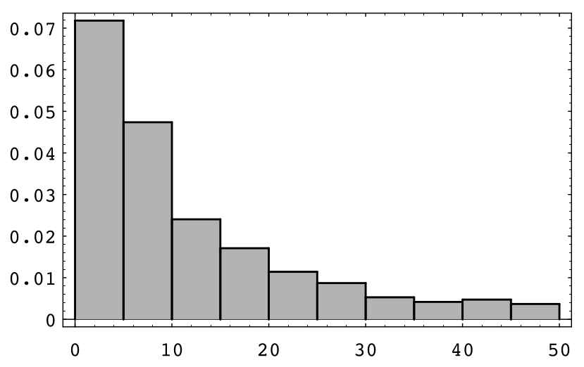
We see that these waiting times appear to be distributed exponentially. This is always the case when $\lambda <\mu$⁠. The proof of this fact is too complicated to give here, but we can verify it by simulation for different choices of $\lambda$ and $\mu$⁠, as above.

Figure 5.7: Queue sizes.

Figure 5.8: Waiting times.

Jones puts in two new lightbulbs: a 60 watt bulb and a 100 watt bulb. It is claimed that the lifetime of the 60 watt bulb has an exponential density with average lifetime 200 hours ($\lambda =1/200$⁠). The 100 watt bulb also has an exponential density but with average lifetime of only 100 hours ($\lambda =1/100$⁠). Jones wonders what is the probability that the 100 watt bulb will outlast the 60 watt bulb.

If $X$ and $Y$ are two independent random variables with exponential densities $f(x)=\lambda e^{-\lambda x}$ and $g(x)=\mu e^{-\mu x}$⁠, respectively, then the probability that $X$ is less than $Y$ is given by $$P(X<Y)={\int }_0^{\infty }f(x)(1-G(x))dx,$$ where $G(x)$ is the cumulative distribution function for $g(x)$⁠. Explain why this is the case. Use this to show that $$P(X<Y)=\frac{\lambda }{\lambda +\mu }$$ and to answer Jones’s question.