Every problem in the chapter beside the book’s answer, a chapter at a time as you scroll.
Chapter 8: Law of Large Numbers
16 problems · 0 figuresExercise 8.1.1 §8.1 source ↗
A fair coin is tossed 100 times. The expected number of heads is 50, and the standard deviation for the number of heads is . What does Chebyshev’s Inequality tell you about the probability that the number of heads that turn up deviates from the expected number 50 by three or more standard deviations (i.e., by at least 15)?
Answer
Exercise 8.1.3 §8.1 source ↗
Write a program to toss a coin 10,000 times. Let be the number of heads in the first tosses. Have your program print out, after every 1000 tosses, . On the basis of this simulation, is it correct to say that you can expect heads about half of the time when you toss a coin a large number of times?
Answer
We shall see that tends to infinity as tends to infinity. While the difference will be small compared to , it will not tend to 0. On the other hand the difference does tend to 0.
Exercise 8.1.5 §8.1 source ↗
Let be a random variable with and . What integer value will assure us that ?
Answer
Exercise 8.1.7 §8.1 source ↗
Find the maximum possible value for if . Using this result and Exercise 6, show that the estimate is valid for any .
Let be the number of successes in Bernoulli trials with probability for success on each trial. Show, using Chebyshev’s Inequality, that for any
Answer
Thus, . From Exercise 6 we have that
Exercise 8.1.9 §8.1 source ↗
In Exercise 6.2.15, you showed that, for the hat check problem, the number of people who get their own hats back has . Using Chebyshev’s Inequality, show that for any .
Suppose that people have their hats returned at random. Let if the th person gets his or her own hat back and 0 otherwise. Let . Then is the total number of people who get their own hats back. Show that
(a) .
(b) for .
(c) (using (a) and (b)).
(d) .
Answer
Exercise 8.1.11 §8.1 source ↗
We have two coins: one is a fair coin and the other is a coin that produces heads with probability 3/4. One of the two coins is picked at random, and this coin is tossed times. Let be the number of heads that turns up in these tosses. Does the Law of Large Numbers allow us to predict the proportion of heads that will turn up in the long run? After we have observed a large number of tosses, can we tell which coin was chosen? How many tosses suffice to make us 95 percent sure?
Answer
No, we cannot predict the proportion of heads that should turn up in the long run, since this will depend upon which of the two coins we pick. If you have observed a large number of trials then, by the Law of Large Numbers, the proportion of heads should be near the probability for the coin that you chose. Thus, in the long run, you will be able to tell which coin you have from the proportion of heads in your observations. To be 95 percent sure, if the proportion of heads is less than , predict ; if it is greater than , predict . Then you will get the correct coin if the proportion of heads does not deviate from the probability of heads by more than . By Exercise 7, the probability of a deviation of this much is less than or equal to . This will be less than or equal to if . Thus with 321 tosses we can be 95 percent sure which coin we have.
Exercise *8.1.15 §8.1 source ↗
We have proved a theorem often called the “Weak Law of Large Numbers." Most people’s intuition and our computer simulations suggest that, if we toss a coin a sequence of times, the proportion of heads will really approach 1/2; that is, if is the number of heads in times, then we will have as . Of course, we cannot be sure of this since we are not able to toss the coin an infinite number of times, and, if we could, the coin could come up heads every time. However, the “Strong Law of Large Numbers," proved in more advanced courses, states that Describe a sample space that would make it possible for us to talk about the event Could we assign the equiprobable measure to this space? (See Example 2.18.)
Consider an experiment in which a fair coin is tossed repeatedly, without stopping. We have seen in Example 1.6 that, for a coin tossed times, the natural sample space is a binary tree with stages. On this evidence we expect that for a coin tossed repeatedly, the natural sample space is a binary tree with an infinite number of stages, as indicated in Figure 2.22.
It is surprising to learn that, although the -stage tree is obviously a finite sample space, the unlimited tree can be described as a continuous sample space. To see how this comes about, let us agree that a typical outcome of the unlimited coin tossing experiment can be described by a sequence of the form . If we write 1 for H and 0 for T, then . In this way, each outcome is described by a sequence of 0’s and 1’s.
Figure 2.22: Tree for infinite number of tosses of a coin.
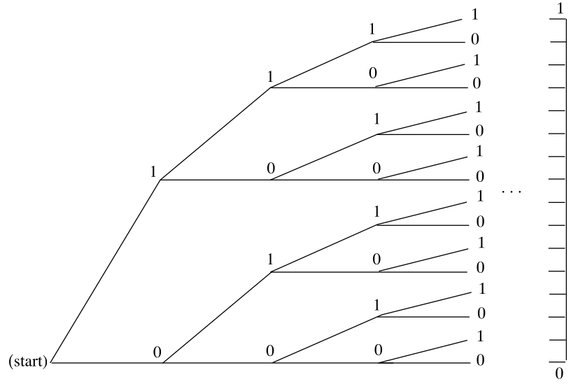
Now suppose we think of this sequence of 0’s and 1’s as the binary expansion of some real number lying between 0 and 1. (A binary expansion is like a decimal expansion but based on 2 instead of 10.) Then each outcome is described by a value of , and in this way becomes a coordinate for the sample space, taking on all real values between 0 and 1. (We note that it is possible for two different sequences to correspond to the same real number; for example, the sequences and both correspond to the real number . We will not concern ourselves with this apparent problem here.)
What probabilities should be assigned to the events of this sample space? Consider, for example, the event consisting of all outcomes for which the first toss comes up heads and the second tails. Every such outcome has the form , where can be either 0 or 1. Now if is our real-valued coordinate, then the value of for every such outcome must lie between and , and moreover, every value of between 1/2 and 3/4 has a binary expansion of the form . This means that if and only if , and in this way we see that we can describe by the interval . More generally, every event consisting of outcomes for which the results of the first tosses are prescribed is described by a binary interval of the form .
We have already seen in Section 1.2 that in the experiment involving tosses, the probability of any one outcome must be exactly . It follows that in the unlimited toss experiment, the probability of any event consisting of outcomes for which the results of the first tosses are prescribed must also be . But is exactly the length of the interval of -values describing ! Thus we see that, just as with the spinner experiment, the probability of an event is determined by what fraction of the unit interval lies in .
Consider again the statement: The probability is 1/2 that a fair coin will turn up heads when tossed. We have suggested that one interpretation of this statement is that if we toss the coin indefinitely the proportion of heads will approach 1/2. That is, in our correspondence with binary sequences we expect to get a binary sequence with the proportion of 1’s tending to 1/2. The event of binary sequences for which this is true is a proper subset of the set of all possible binary sequences. It does not contain, for example, the sequence (i.e., (011) repeated again and again). The event is actually a very complicated subset of the binary sequences, but its probability can be determined as a limit of probabilities for events with a finite number of outcomes whose probabilities are given by finite tree measures. When the probability of is computed in this way, its value is found to be 1. This remarkable result is known as the Strong Law of Large Numbers (or Law of Averages) and is one justification for our frequency concept of probability. We shall prove a weak form of this theorem in Chapter 8.
A die is rolled once. We let denote the outcome of this experiment. Then the sample space for this experiment is the 6-element set where each outcome , for , …, 6, corresponds to the number of dots on the face which turns up. The event corresponds to the statement that the result of the roll is an even number. The event can also be described by saying that is even. Unless there is reason to believe the die is loaded, the natural assumption is that every outcome is equally likely. Adopting this convention means that we assign a probability of 1/6 to each of the six outcomes, i.e., , for .
Figure 2.22: Tree for infinite number of tosses of a coin.
Answer
Take as the set of all sequences of 0’s and 1’s, with 1’s indicating heads and 0’s indicating tails. We cannot determine a probability distribution by simply assigning equal weights to all infinite sequences, since these weights would have to be 0. Instead, we assign probabilities to finite sequences in the usual way, and then probabilities of events that depend on infinite sequences can be obtained as limits of these finite sequences. (See Exercise 28 of Chapter 1, Section 1.2.)
Exercise *8.1.17 §8.1 source ↗
Let us toss a biased coin that comes up heads with probability and assume the validity of the Strong Law of Large Numbers as described in Exercise 15. Then, with probability 1, as . If is a continuous function on the unit interval, then we also have
Finally, we could hope that Show that, if all this is correct, as in fact it is, we would have proven that any continuous function on the unit interval is a limit of polynomial functions. This is a sketch of a probabilistic proof of an important theorem in mathematics called the Weierstrass approximation theorem.
We have proved a theorem often called the “Weak Law of Large Numbers." Most people’s intuition and our computer simulations suggest that, if we toss a coin a sequence of times, the proportion of heads will really approach 1/2; that is, if is the number of heads in times, then we will have as . Of course, we cannot be sure of this since we are not able to toss the coin an infinite number of times, and, if we could, the coin could come up heads every time. However, the “Strong Law of Large Numbers," proved in more advanced courses, states that Describe a sample space that would make it possible for us to talk about the event Could we assign the equiprobable measure to this space? (See Example 2.18.)
Consider an experiment in which a fair coin is tossed repeatedly, without stopping. We have seen in Example 1.6 that, for a coin tossed times, the natural sample space is a binary tree with stages. On this evidence we expect that for a coin tossed repeatedly, the natural sample space is a binary tree with an infinite number of stages, as indicated in Figure 2.22.
It is surprising to learn that, although the -stage tree is obviously a finite sample space, the unlimited tree can be described as a continuous sample space. To see how this comes about, let us agree that a typical outcome of the unlimited coin tossing experiment can be described by a sequence of the form . If we write 1 for H and 0 for T, then . In this way, each outcome is described by a sequence of 0’s and 1’s.
Figure 2.22: Tree for infinite number of tosses of a coin.
Now suppose we think of this sequence of 0’s and 1’s as the binary expansion of some real number lying between 0 and 1. (A binary expansion is like a decimal expansion but based on 2 instead of 10.) Then each outcome is described by a value of , and in this way becomes a coordinate for the sample space, taking on all real values between 0 and 1. (We note that it is possible for two different sequences to correspond to the same real number; for example, the sequences and both correspond to the real number . We will not concern ourselves with this apparent problem here.)
What probabilities should be assigned to the events of this sample space? Consider, for example, the event consisting of all outcomes for which the first toss comes up heads and the second tails. Every such outcome has the form , where can be either 0 or 1. Now if is our real-valued coordinate, then the value of for every such outcome must lie between and , and moreover, every value of between 1/2 and 3/4 has a binary expansion of the form . This means that if and only if , and in this way we see that we can describe by the interval . More generally, every event consisting of outcomes for which the results of the first tosses are prescribed is described by a binary interval of the form .
We have already seen in Section 1.2 that in the experiment involving tosses, the probability of any one outcome must be exactly . It follows that in the unlimited toss experiment, the probability of any event consisting of outcomes for which the results of the first tosses are prescribed must also be . But is exactly the length of the interval of -values describing ! Thus we see that, just as with the spinner experiment, the probability of an event is determined by what fraction of the unit interval lies in .
Consider again the statement: The probability is 1/2 that a fair coin will turn up heads when tossed. We have suggested that one interpretation of this statement is that if we toss the coin indefinitely the proportion of heads will approach 1/2. That is, in our correspondence with binary sequences we expect to get a binary sequence with the proportion of 1’s tending to 1/2. The event of binary sequences for which this is true is a proper subset of the set of all possible binary sequences. It does not contain, for example, the sequence (i.e., (011) repeated again and again). The event is actually a very complicated subset of the binary sequences, but its probability can be determined as a limit of probabilities for events with a finite number of outcomes whose probabilities are given by finite tree measures. When the probability of is computed in this way, its value is found to be 1. This remarkable result is known as the Strong Law of Large Numbers (or Law of Averages) and is one justification for our frequency concept of probability. We shall prove a weak form of this theorem in Chapter 8.
A die is rolled once. We let denote the outcome of this experiment. Then the sample space for this experiment is the 6-element set where each outcome , for , …, 6, corresponds to the number of dots on the face which turns up. The event corresponds to the statement that the result of the roll is an even number. The event can also be described by saying that is even. Unless there is reason to believe the die is loaded, the natural assumption is that every outcome is equally likely. Adopting this convention means that we assign a probability of 1/6 to each of the six outcomes, i.e., , for .
Figure 2.22: Tree for infinite number of tosses of a coin.
Answer
For , let us toss a biased coin that comes up heads with probability . Then But The right side is a polynomial, and the left side tends to . Hence This shows that we can obtain obtain any continuous function on as a limit of polynomial functions.
Exercise 8.2.1 §8.2 source ↗
Let be a continuous random variable with mean and variance . Using Chebyshev’s Inequality, find an upper bound for the following probabilities.
(a) .
(b) .
(c) .
(d) .
Answer
(a)
(b)
(c)
(d)
Exercise 8.2.3 §8.2 source ↗
Let be the random variable of Exercise 2.
(a) Calculate the function .
(b) Now graph the function , and on the same axes, graph the Chebyshev function . Show that for all , but that is not a very good approximation for .
Let be a continuous random variable with values unformly distributed over the interval .
(a) Find the mean and variance of .
(b) Calculate , , , and exactly. How do your answers compare with those of Exercise 1? How good is Chebyshev’s Inequality in this case?
Let be a continuous random variable with mean and variance . Using Chebyshev’s Inequality, find an upper bound for the following probabilities.
(a) .
(b) .
(c) .
(d) .
Answer
Exercise 8.2.5 §8.2 source ↗
Let be a continuous random variable with values normally distributed over with mean and variance .
(a) Using Chebyshev’s Inequality, find upper bounds for the following probabilities: , , and .
(b) The area under the normal curve between and 1 is .6827, between and 2 is .9545, and between and 3 it is .9973 (see the table in Appendix A). Compare your bounds in (a) with these exact values. How good is Chebyshev’s Inequality in this case?
Answer
(a) , ,
(b) vs. , vs. , vs.
Exercise 8.2.7 §8.2 source ↗
If is a random variable with mean and variance , define the relative deviation of from its mean by
(a) Show that .
(b) If is the random variable of Exercise 1, find an upper bound for , , , and .
Let be a continuous random variable with mean and variance . Using Chebyshev’s Inequality, find an upper bound for the following probabilities.
(a) .
(b) .
(c) .
(d) .
Answer
(b) , , ,
Exercise 8.2.9 §8.2 source ↗
(a) Suppose a number is chosen at random from with uniform probability. Find a lower bound for the probability that lies between 8 and 12, using Chebyshev’s Inequality.
(b) Now suppose 20 real numbers are chosen independently from with uniform probability. Find a lower bound for the probability that their average lies between 8 and 12.
(c) Now suppose 100 real numbers are chosen independently from . Find a lower bound for the probability that their average lies between 8 and 12.
Answer
(a)
(b)
(c)
Exercise 8.2.11 §8.2 source ↗
The Pilsdorff beer company runs a fleet of trucks along the 100 mile road from Hangtown to Dry Gulch, and maintains a garage halfway in between. Each of the trucks is apt to break down at a point miles from Hangtown, where is a random variable uniformly distributed over .
(a) Find a lower bound for the probability .
(b) Suppose that in one bad week, 20 trucks break down. Find a lower bound for the probability , where is the average of the distances from Hangtown at the time of breakdown.
Answer
(a)
(b)
Exercise 8.2.13 §8.2 source ↗
Suppose one hundred numbers , , …, are chosen independently at random from . Let be the sum, the average, and the standardized sum. Find lower bounds for the probabilities
(a) .
(b) .
(c) .
Answer
(a)
(b)
(c)
Exercise 8.2.17 §8.2 source ↗
Show that, if , then .
Answer
. Since is non-negative, we have
Loading chapter 9…
Exercises and answers are adapted from Grinstead and Snell's Introduction to Probability by The CHANCE Project, which is free to read and download, and are used under the GNU FDL licence. They are taken from the GNU version’s LaTeX source (4 July 2006), with answers from the authors’ published answers to the odd-numbered exercises, and set for the web, so they may differ slightly from the printed page. This adaptation is released under the same licence and is neither affiliated with nor endorsed by Grinstead and Snell or American Mathematical Society. Copyright (C) 2006 Peter G. Doyle. This work is a version of Grinstead and Snell's ‘Introduction to Probability, 2nd edition’, published by the American Mathematical Society, Copyright (C) 2003 Charles M. Grinstead and J. Laurie Snell.