Chapter 6: Expected Value and VarianceContent check — Probability (Grinstead and Snell), Chapter 6: Expected Value and Variance

In Las Vegas, a roulette wheel has 38 slots numbered 0, 00, 1, 2, …, 36. The 0 and 00 slots are green and half of the remaining 36 slots are red and half are black. A croupier spins the wheel and throws in an ivory ball. If you bet 1 dollar on red, you win 1 dollar if the ball stops in a red slot and otherwise you lose 1 dollar. Write a program to find the total winnings for a player who makes 1000 bets on red.

Another form of bet for roulette is to bet that a specific number (say 17) will turn up. If the ball stops on your number, you get your dollar back plus 35 dollars. If not, you lose your dollar. Write a program that will plot your winnings when you make 500 plays of roulette at Las Vegas, first when you bet each time on red (see Exercise 6), and then for a second visit to Las Vegas when you make 500 plays betting each time on the number 17. What differences do you see in the graphs of your winnings on these two occasions?

(Heads or Tails) For our next example, we consider a problem where the exact answer is difficult to obtain but for which simulation easily gives the qualitative results. Peter and Paul play a game called heads or tails. In this game, a fair coin is tossed a sequence of times—we choose 40. Each time a head comes up Peter wins 1 penny from Paul, and each time a tail comes up Peter loses 1 penny to Paul. For example, if the results of the 40 tosses are

THTHHHHTTHTHHTTHHTTTTHHHTHHTHHHTHHHTTTHH.

Peter’s winnings may be graphed as in Figure 1.1.
Figure 1.1: Peter’s winnings in 40 plays of heads or tails.

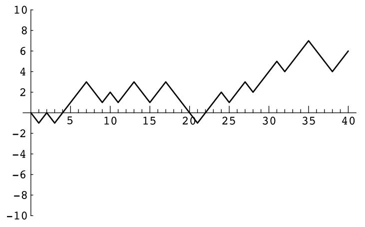
Peter has won 6 pennies in this particular game. It is natural to ask for the probability that he will win $j$ pennies; here $j$ could be any even number from $-40$ to $40$⁠. It is reasonable to guess that the value of $j$ with the highest probability is $j=0$⁠, since this occurs when the number of heads equals the number of tails. Similarly, we would guess that the values of $j$ with the lowest probabilities are $j=\pm 40$⁠.

A second interesting question about this game is the following: How many times in the 40 tosses will Peter be in the lead? Looking at the graph of his winnings (Figure 1.1), we see that Peter is in the lead when his winnings are positive, but we have to make some convention when his winnings are 0 if we want all tosses to contribute to the number of times in the lead. We adopt the convention that, when Peter’s winnings are 0, he is in the lead if he was ahead at the previous toss and not if he was behind at the previous toss. With this convention, Peter is in the lead 34 times in our example. Again, our intuition might suggest that the most likely number of times to be in the lead is 1/2 of 40, or 20, and the least likely numbers are the extreme cases of 40 or 0.

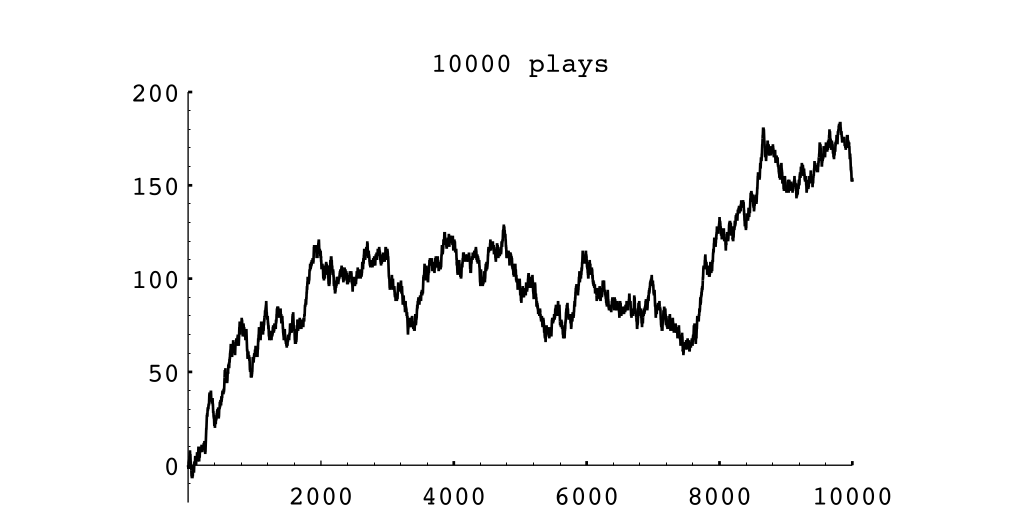
It is easy to settle this by simulating the game a large number of times and keeping track of the number of times that Peter’s final winnings are $j$⁠, and the number of times that Peter ends up being in the lead by $k$⁠. The proportions over all games then give estimates for the corresponding probabilities. The program HTSimulation carries out this simulation. Note that when there are an even number of tosses in the game, it is possible to be in the lead only an even number of times. We have simulated this game 10,000 times. The results are shown in Figures 1.2 and 1.3. These graphs, which we call spike graphs, were generated using the program Spikegraph. The vertical line, or spike, at position $x$ on the horizontal axis, has a height equal to the proportion of outcomes which equal $x$⁠. Our intuition about Peter’s final winnings was quite correct, but our intuition about the number of times Peter was in the lead was completely wrong. The simulation suggests that the least likely number of times in the lead is 20 and the most likely is 0 or 40. This is indeed correct, and the explanation for it is suggested by playing the game of heads or tails with a large number of tosses and looking at a graph of Peter’s winnings. In Figure 1.4 we show the results of a simulation of the game, for 1000 tosses and in Figure 1.5 for 10,000 tosses.

In the second example Peter was ahead most of the time. It is a remarkable fact, however, that, if play is continued long enough, Peter’s winnings will continue to come back to 0, but there will be very long times between the times that this happens. These and related results will be discussed in Chapter 12.

Figure 1.1: Peter’s winnings in 40 plays of heads or tails.

Figure 1.2: Distribution of winnings.

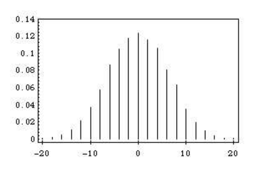
Figure 1.3: Distribution of number of times in the lead.

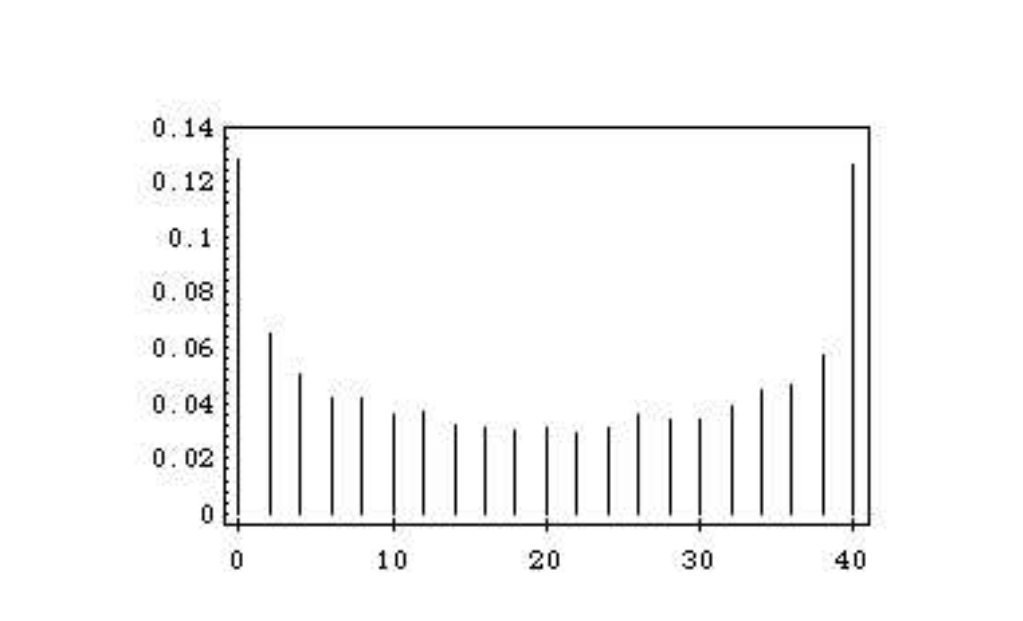
Figure 1.4: Peter’s winnings in 1000 plays of heads or tails.

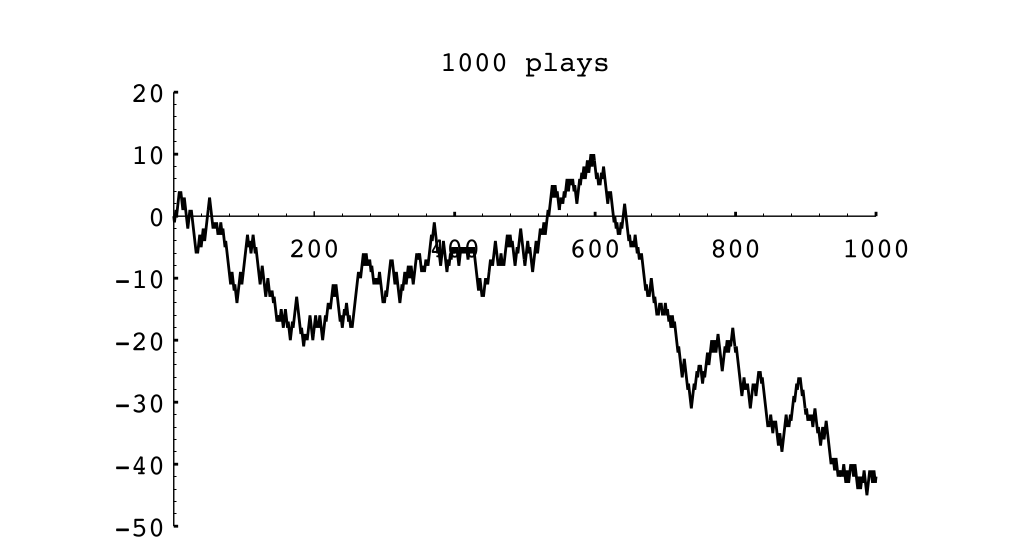
Figure 1.5: Peter’s winnings in 10,000 plays of heads or tails.

Assume that, every time you buy a box of Wheaties, you receive a picture of one of the $n$ players for the New York Yankees (see Exercise 3.2.34). Let $X_k$ be the number of additional boxes you have to buy, after you have obtained $k-1$ different pictures, in order to obtain the next new picture. Thus $X_1=1$⁠, $X_2$ is the number of boxes bought after this to obtain a picture different from the first pictured obtained, and so forth.

(a) Show that $X_k$ has a geometric distribution with $p=(n-k+1)/n$⁠.

(b) Simulate the experiment for a team with 26 players (25 would be more accurate but we want an even number). Carry out a number of simulations and estimate the expected time required to get the first 13 players and the expected time to get the second 13. How do these expectations compare?

(c) Show that, if there are $2n$ players, the expected time to get the first half of the players is $$2n(\frac{1}{2n}+\frac{1}{2n-1}+\cdots +\frac{1}{n+1}),$$ and the expected time to get the second half is $$2n(\frac{1}{n}+\frac{1}{n-1}+\cdots +1).$$

(d) In Example 6.11 we stated that $$1+\frac{1}{2}+\frac{1}{3}+\cdots +\frac{1}{n}\sim \log n+.5772+\frac{1}{2n}.$$ Use this to estimate the expression in (c). Compare these estimates with the exact values and also with your estimates obtained by simulation for the case $n=26$⁠.

Assume that every time you buy a box of Wheaties, you receive one of the pictures of the $n$ players on the New York Yankees. Over a period of time, you buy $m\ge n$ boxes of Wheaties.

(a) Use Theorem 3.8 to show that the probability that you get all $n$ pictures is
$$\begin{array}{ccc}\hfill 1& -\hfill & \hfill \left(\frac{n}{1}\right){\left(\frac{n-1}{n}\right)}^m+\left(\frac{n}{2}\right){\left(\frac{n-2}{n}\right)}^m-\cdots \\ \hfill & +\hfill & \hfill {(-1)}^{n-1}\left(\frac{n}{n-1}\right){\left(\frac{1}{n}\right)}^m.\end{array}$$
Hint: Let $E_k$ be the event that you do not get the $k$⁠th player’s picture.

(b) Write a computer program to compute this probability. Use this program to find, for given $n$⁠, the smallest value of $m$ which will give probability $\ge .5$ of getting all $n$ pictures. Consider $n=50$⁠, 100, and 150 and show that $m=n\log n+n\log 2$ is a good estimate for the number of boxes needed. (For a derivation of this estimate, see Feller. (W. Feller, Introduction to Probability Theory and its Applications, vol. I, 3rd ed. (New York: John Wiley & Sons, 1968), p. 106.))

Let $P$ be a probability distribution on a sample space $\mathrm{\Omega }$⁠, and let $\{A_1,A_2,\dots ,A_n\}$ be a finite set of events. Then $$P(A_1\cup A_2\cup \cdots \cup A_n)=\sum _{i=1}^{n}P(A_i)-\sum _{1\le i<j\le n}P(A_i\cap A_j)$$

$$+\sum _{1\le i<j<k\le n}P(A_i\cap A_j\cap A_k)-\cdots .$$

That is, to find the probability that at least one of $n$ events $A_i$ occurs, first add the probability of each event, then subtract the probabilities of all possible two-way intersections, add the probability of all three-way intersections, and so forth. Proof. If the outcome $\omega$ occurs in at least one of the events $A_i$⁠, its probability is added exactly once by the left side of Equation 3.3. We must show that it is added exactly once by the right side of Equation 3.3. Assume that $\omega$ is in exactly $k$ of the sets. Then its probability is added $k$ times in the first term, subtracted $\left(\frac{k}{2}\right)$ times in the second, added $\left(\frac{k}{3}\right)$ times in the third term, and so forth. Thus, the total number of times that it is added is $$\left(\frac{k}{1}\right)-\left(\frac{k}{2}\right)+\left(\frac{k}{3}\right)-\cdots {(-1)}^{k-1}\left(\frac{k}{k}\right).$$ But $$0={(1-1)}^k=\sum _{j=0}^k\left(\frac{k}{j}\right){(-1)}^j=\left(\frac{k}{0}\right)-\sum _{j=1}^k\left(\frac{k}{j}\right){(-1)}^{j-1}.$$ Hence, $$1=\left(\frac{k}{0}\right)=\sum _{j=1}^k\left(\frac{k}{j}\right){(-1)}^{j-1}.$$ If the outcome $\omega$ is not in any of the events $A_i$⁠, then it is not counted on either side of the equation.

$$+\sum _{1\le i<j<k\le n}P(A_i\cap A_j\cap A_k)-\cdots .$$

We start keeping snowfall records this year and want to find the expected number of records that will occur in the next $n$ years. The first year is necessarily a record. The second year will be a record if the snowfall in the second year is greater than that in the first year. By symmetry, this probability is 1/2. More generally, let $X_j$ be 1 if the $j$⁠th year is a record and 0 otherwise. To find $E(X_j)$⁠, we need only find the probability that the $j$⁠th year is a record. But the record snowfall for the first $j$ years is equally likely to fall in any one of these years, so $E(X_j)=1/j$⁠. Therefore, if $S_n$ is the total number of records observed in the first $n$ years, $$E(S_n)=1+\frac{1}{2}+\frac{1}{3}+\cdots +\frac{1}{n}.$$ This is the famous divergent harmonic series. It is easy to show that $$E(S_n)\sim \log n$$ as $n\to \infty$⁠. A more accurate approximation to $E(S_n)$ is given by the expression $$\log n+\gamma +\frac{1}{2n},$$ where $\gamma$ denotes Euler’s constant, and is approximately equal to .5772.

Therefore, in ten years the expected number of records is approximately $2.9298$⁠; the exact value is the sum of the first ten terms of the harmonic series which is 2.9290.

Let $X$ be a random variable with range $[-\mathrm{1,1}]$ and density function $f_X(x)=ax+b$ if $|x|<1$⁠.

(a) Show that if ${\int }_{-1}^{+1}{f}_X(x)dx=1$⁠, then $b=1/2$⁠.

(b) Show that if $f_X(x)\ge 0$⁠, then $-1/2\le a\le 1/2$⁠.

(c) Show that $\mu =(2/3)a$⁠, and hence that $-1/3\le \mu \le 1/3$⁠.

(d) Show that ${\sigma }^2(X)=$ $(2/3)b-$ $(4/9)a^2=$ $1/3-$ $(4/9)a^2$⁠.

If $X$ and $Y$ are any two random variables, then the covariance of $X$ and $Y$ is defined by Cov⁠$(X,Y)=$ $E((X-E(X))(Y-E(Y)))$⁠. Note that Cov⁠$(X,X)=V(X)$⁠. Show that, if $X$ and $Y$ are independent, then Cov⁠$(X,Y)=0$⁠; and show, by an example, that we can have Cov⁠$(X,Y)=0$ and $X$ and $Y$ not independent.

Let $X$ and $Y$ be random variables with positive variance. The correlation of $X$ and $Y$ is defined as $$\rho (X,Y)=\frac{\mathrm{cov}(X,Y)}{\sqrt{V(X)V(Y)}}.$$

(a) Using Exercise 17(c), show that $$0\le V(\frac{X}{\sigma (X)}+\frac{Y}{\sigma (Y)})=2(1+\rho (X,Y)).$$

(b) Now show that $$0\le V(\frac{X}{\sigma (X)}-\frac{Y}{\sigma (Y)})=2(1-\rho (X,Y)).$$

(c) Using (a) and (b), show that $$-1\le \rho (X,Y)\le 1.$$

Let $X$ and $Y$ be random variables. The covariance $\mathrm{C}\mathrm{o}\mathrm{v}(\mathrm{X},\mathrm{Y})$ is defined by (see Exercise 6.2.23) $$\mathrm{c}\mathrm{o}\mathrm{v}(\mathrm{X},\mathrm{Y})=\mathrm{E}((\mathrm{X}-\mathrm{\mu }(\mathrm{X}))(\mathrm{Y}-\mathrm{\mu }(\mathrm{Y}))).$$

(a) Show that $\mathrm{c}\mathrm{o}\mathrm{v}(\mathrm{X},\mathrm{Y})=\mathrm{E}(\mathrm{X}\mathrm{Y})-\mathrm{E}(\mathrm{X})\mathrm{E}(\mathrm{Y})$⁠.

(b) Using (a), show that $\mathrm{cov}(X,Y)=0$⁠, if $X$ and $Y$ are independent. (Caution: the converse is not always true.)

(c) Show that $V(X+Y)=$ $V(X)+$ $V(Y)+$ $2\mathrm{cov}(X,Y)$⁠.

If $X$ and $Y$ are any two random variables, then the covariance of $X$ and $Y$ is defined by Cov⁠$(X,Y)=$ $E((X-E(X))(Y-E(Y)))$⁠. Note that Cov⁠$(X,X)=V(X)$⁠. Show that, if $X$ and $Y$ are independent, then Cov⁠$(X,Y)=0$⁠; and show, by an example, that we can have Cov⁠$(X,Y)=0$ and $X$ and $Y$ not independent.