Every problem in the chapter beside the book’s answer, a chapter at a time as you scroll.
Chapter 9: Central Limit Theorem
11 problems · 0 figuresExercise 9.1.1 §9.1 source ↗
Let be the number of heads that turn up in 100 tosses of a fair coin. Use the Central Limit Theorem to estimate
(a) .
(b) .
(c) .
(d) .
Answer
(a)
(b)
(c)
(d)
(The answers to the problems in this chapter do not use the ‘1/2 correction mentioned in Section 9.1.
Exercise 9.1.3 §9.1 source ↗
A true-false examination has 48 questions. June has probability 3/4 of answering a question correctly. April just guesses on each question. A passing score is 30 or more correct answers. Compare the probability that June passes the exam with the probability that April passes it.
Answer
(a)
(b)
(The answers to the problems in this chapter do not use the ‘1/2 correction mentioned in Section 9.1.
Exercise 9.1.5 §9.1 source ↗
A rookie is brought to a baseball club on the assumption that he will have a .300 batting average. (Batting average is the ratio of the number of hits to the number of times at bat.) In the first year, he comes to bat 300 times and his batting average is .267. Assume that his at bats can be considered Bernoulli trials with probability .3 for success. Could such a low average be considered just bad luck or should he be sent back to the minor leagues? Comment on the assumption of Bernoulli trials in this situation.
Answer
Since his batting average was , he must have had 80 hits. The probability that one would obtain 80 or fewer successes in 300 Bernoulli trials, with individual probability of success , is approximately . Thus, the low average is probably not due to bad luck (but a statistician would not reject the hypothesis that the player has a probability of success equal to ).
(The answers to the problems in this chapter do not use the ‘1/2 correction mentioned in Section 9.1.
Exercise 9.1.7 §9.1 source ↗
Assume that, as in Example 9.3, Dartmouth admits 1750 students. What is the probability of too many acceptances?
Dartmouth College would like to have 1050 freshmen. This college cannot accommodate more than 1060. Assume that each applicant accepts with probability .6 and that the acceptances can be modeled by Bernoulli trials. If the college accepts 1700, what is the probability that it will have too many acceptances?
If it accepts 1700 students, the expected number of students who matriculate is . The standard deviation for the number that accept is . Thus we want to estimate the probability
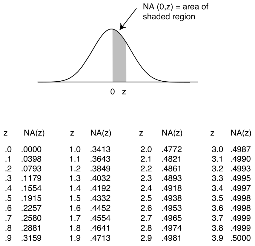
From Table 9.4, if we interpolate, we would estimate this probability to be . Thus, the college is fairly safe using this admission policy.
Figure 9.4: Table of values of , the normal area from 0 to .
Answer
(The answers to the problems in this chapter do not use the ‘1/2 correction mentioned in Section 9.1.
Exercise 9.1.9 §9.1 source ↗
Let be the number of successes in Bernoulli trials with probability .8 for success on each trial. Let be the average number of successes. In each case give the value for the limit, and give a reason for your answer.
(a) .
(b) .
(c) .
(d) .
Answer
(a)
(b) (Law of Large Numbers)
(c) (Central Limit Theorem)
(d) (Law of Large Numbers)
(The answers to the problems in this chapter do not use the ‘1/2 correction mentioned in Section 9.1.
Exercise 9.1.13 §9.1 source ↗
A noodle machine in Spumoni’s spaghetti factory makes about 5 percent defective noodles even when properly adjusted. The noodles are then packed in crates containing 1900 noodles each. A crate is examined and found to contain 115 defective noodles. What is the approximate probability of finding at least this many defective noodles if the machine is properly adjusted?
Answer
(The answers to the problems in this chapter do not use the ‘1/2 correction mentioned in Section 9.1.
Exercise 9.1.17 §9.1 source ↗
In an opinion poll it is assumed that an unknown proportion of the people are in favor of a proposed new law and a proportion are against it. A sample of people is taken to obtain their opinion. The proportion in favor in the sample is taken as an estimate of . Using the Central Limit Theorem, determine how large a sample will ensure that the estimate will, with probability .95, be correct to within .01.
Answer
We want . Replacing by its upper bound , we have . Thus we would need . Recall that by Chebyshev’s inequality we would need .
(The answers to the problems in this chapter do not use the ‘1/2 correction mentioned in Section 9.1.
Exercise 9.3.1 §9.3 source ↗
Let be a continuous random variable with mean and variance , and let be its standardized version. Verify directly that and .
Answer
(The answers to the problems in this chapter do not use the ‘1/2 correction mentioned in Section 9.1.
Exercise 9.3.3 §9.3 source ↗
Let , , be a sequence of random variables, all with mean and variance , and be their standardized versions. Let and be the sum of the and , and and their standardized version. Show that .
Answer
. Since each has mean 0 and variance 1, and . Thus .
(The answers to the problems in this chapter do not use the ‘1/2 correction mentioned in Section 9.1.
Exercise 9.3.11 §9.3 source ↗
The price of one share of stock in the Pilsdorff Beer Company (see Exercise 8.2.12) is given by on the th day of the year. Finn observes that the differences appear to be independent random variables with a common distribution having mean and variance . If , estimate the probability that is
(a) .
(b) .
(c) .
A share of common stock in the Pilsdorff beer company has a price on the th business day of the year. Finn observes that the price change appears to be a random variable with mean and variance . If , find a lower bound for the following probabilities, under the assumption that the ’s are mutually independent.
(a) .
(b) .
(c) .
Answer
(a)
(b)
(c)
(The answers to the problems in this chapter do not use the ‘1/2 correction mentioned in Section 9.1.
Exercise 9.3.13 §9.3 source ↗
Physicists say that particles in a long tube are constantly moving back and forth along the tube, each with a velocity (in cm/sec) at any given moment that is normally distributed, with mean and variance . Suppose there are particles in the tube.
(a) Find the mean and variance of the average velocity of the particles.
(b) What is the probability that the average velocity is cm/sec?
Answer
(The answers to the problems in this chapter do not use the ‘1/2 correction mentioned in Section 9.1.
Loading chapter 10…
Exercises and answers are adapted from Grinstead and Snell's Introduction to Probability by The CHANCE Project, which is free to read and download, and are used under the GNU FDL licence. They are taken from the GNU version’s LaTeX source (4 July 2006), with answers from the authors’ published answers to the odd-numbered exercises, and set for the web, so they may differ slightly from the printed page. This adaptation is released under the same licence and is neither affiliated with nor endorsed by Grinstead and Snell or American Mathematical Society. Copyright (C) 2006 Peter G. Doyle. This work is a version of Grinstead and Snell's ‘Introduction to Probability, 2nd edition’, published by the American Mathematical Society, Copyright (C) 2003 Charles M. Grinstead and J. Laurie Snell.