Every problem in the chapter beside the book’s answer, a chapter at a time as you scroll.
Chapter 1: Linear Systems
153 problems · 16 figuresOne.I.1.17 §I.1 source ↗
Use Gauss’s Method to find the unique solution for each system.
Answer (2 parts)
Gauss’s Method
gives that the solution is and .
Gauss’s Method here
gives , , and .
One.I.1.18 §I.1 source ↗
Each system is in echelon form. For each, say whether the system has a unique solution, no solution, or infinitely many solutions.
Answer (11 parts)
If a system has a contradictory equation then it has no solution. Otherwise, if there are any variables that are not leading a row then it has infinitely many solution. In the final case, where there is no contradictory equation and every variable leads some row, it has a unique solution.
Unique solution
Infinitely many solutions
Infinitely many solutions
No solution
Infinitely many solutions
Infinitely many solutions
No solution
Infinitely many solutions
No solution
Unique solution
One.I.1.19 §I.1 source ↗
Use Gauss’s Method to solve each system or conclude ‘many solutions’ or ‘no solutions’.
Answer (6 parts)
Gaussian reduction
shows that and is the unique solution.
Gauss’s Method
gives and as the only solution.
Row reduction
shows, because the variable is not a leading variable in any row, that there are many solutions.
Row reduction
shows that there is no solution.
Gauss’s Method
gives the unique solution .
Here Gauss’s Method gives
which shows that there are many solutions.
One.I.1.20 §I.1 source ↗
Solve each system or conclude ‘many solutions’ or ‘no solutions’. Use Gauss’s Method.
Answer (3 parts)
Gauss’s Method
followed by back-substitution gives , , and .
Here Gauss’s Method
finds that the variable does not lead a row. There are infinitely many solutions.
The steps
give .
One.I.1.21 §I.1 source ↗
We can solve linear systems by methods other than Gauss’s. One often taught in high school is to solve one of the equations for a variable, then substitute the resulting expression into other equations. Then we repeat that step until there is an equation with only one variable. From that we get the first number in the solution and then we get the rest with back-substitution. This method takes longer than Gauss’s Method, since it involves more arithmetic operations, and is also more likely to lead to errors. To illustrate how it can lead to wrong conclusions, we will use the system
from Example 1.13.
Solve the first equation for and substitute that expression into the second equation. Find the resulting .
Again solve the first equation for , but this time substitute that expression into the third equation. Find this .
What extra step must a user of this method take to avoid erroneously concluding a system has a solution?
Answer (3 parts)
From we get that , giving .
From we get that , leading to the conclusion that .
Users of this method must check any potential solutions by substituting back into all the equations.
One.I.1.22 §I.1 source ↗
For which values of are there no solutions, many solutions, or a unique solution to this system?
Answer
Do the reduction
to conclude this system has no solutions if and if then it has infinitely many solutions. It never has a unique solution.
One.I.1.23 §I.1 source ↗
This system is not linear in that it says instead of
and yet we can apply Gauss’s Method. Do so. Does the system have a solution?
Answer
Let , , and :
gives , , and . Note that no satisfies that .
One.I.1.24 §I.1 source ↗
What conditions must the constants, the ’s, satisfy so that each of these systems has a solution? Hint. Apply Gauss’s Method and see what happens to the right side.
Answer (2 parts)
Gauss’s Method
shows that this system is consistent if and only if both and .
Reduction
shows that each of , , and can be any real number — this system always has a unique solution.
One.I.1.25 §I.1 source ↗
True or false: a system with more unknowns than equations has at least one solution. (As always, to say ‘true’ you must prove it, while to say ‘false’ you must produce a counterexample.)
Answer
This system with more unknowns than equations
has no solution.
One.I.1.26 §I.1 source ↗
Must any Chemistry problem like the one that starts this subsection — a balance the reaction problem — have infinitely many solutions?
Answer
Yes. For example, the fact that we can have the same reaction in two different flasks shows that twice any solution is another, different, solution (if a physical reaction occurs then there must be at least one nonzero solution).
One.I.1.27 §I.1 source ↗
Find the coefficients , , and so that the graph of passes through the points , , and .
Answer
Because , , and we get a linear system.
Gauss’s Method
shows that the solution is .
One.I.1.28 §I.1 source ↗
After Theorem 1.5 we note that multiplying a row by is not allowed because that could change a solution set. Give an example of a system with solution set where after multiplying a row by the new system has a solution set and is a proper subset of , that is, . Give an example where .
Answer
Here
while is a proper superset because it contains at least two points: and . In this example the solution set does not change.
One.I.1.29 §I.1 source ↗
Gauss’s Method works by combining the equations in a system to make new equations.
Can we derive the equation by a sequence of Gaussian reduction steps from the equations in this system?
Can we derive the equation with a sequence of Gaussian reduction steps from the equations in this system?
Can we derive by a sequence of Gaussian reduction steps from the equations in the system?
Answer (3 parts)
Yes, by inspection the given equation results from .
No. The pair satisfies the given equation. However, that pair does not satisfy the first equation in the system.
Yes. To see if the given row is , solve the system of equations relating the coefficients of , , , and the constants:
and get and , so the given row is .
One.I.1.30 §I.1 source ↗
Prove that, where are real numbers with , if this linear equation
has the same solution set as this one
then they are the same equation. What if ?
Answer
If then the solution set of the first equation is this.
Thus, given we can compute the associated . Taking gives the solution , and since the second equation is supposed to have the same solution set, substituting into it gives that , so . Taking in () gives , and so . Hence they are the same equation.
When the equations can be different and still have the same solution set: e.g., and .
One.I.1.31 §I.1 source ↗
Show that if then
has a unique solution.
Answer
We take three cases: that , that and , and that both and .
For the first, we assume that . Then the reduction
shows that this system has a unique solution if and only if ; remember that so that back substitution yields a unique (observe, by the way, that and play no role in the conclusion that there is a unique solution, although if there is a unique solution then they contribute to its value). But and a fraction is not equal to if and only if its numerator is not equal to . Thus, in this first case, there is a unique solution if and only if .
In the second case, if but , then we swap
to conclude that the system has a unique solution if and only if (we use the case assumption that to get a unique in back substitution). But — where and — the condition “” is equivalent to the condition “”. That finishes the second case.
Finally, for the third case, if both and are then the system
might have no solutions (if the second equation is not a multiple of the first) or it might have infinitely many solutions (if the second equation is a multiple of the first then for each satisfying both equations, any pair will do), but it never has a unique solution. Note that and gives that .
One.I.1.32 §I.1 source ↗
In the system
each of the equations describes a line in the -plane. By geometrical reasoning, show that there are three possibilities: there is a unique solution, there is no solution, and there are infinitely many solutions.
Answer
Recall that if a pair of lines share two distinct points then they are the same line. That’s because two points determine a line, so these two points determine each of the two lines, and so they are the same line.
Thus the lines can share one point (giving a unique solution), share no points (giving no solutions), or share at least two points (which makes them the same line).
One.I.1.33 §I.1 source ↗
Finish the proof of Theorem 1.5.
Answer
For the reduction operation of multiplying by a nonzero real number , we have that satisfies this system
if and only if and … and … by the definition of ‘satisfies’. Because , that’s true if and only if and … and … (this is straightforward canceling on both sides of the -th equation), which says that solves
as required.
For the combination operation , the tuple satisfies
if and only if and … and … and … again by the definition of ‘satisfies’. Subtract times the equation from equation . (Here is where we need ; if then the two ’s above are not equal.) The previous compound statement holds if and only if and … and… and… , which after cancellation says that solves
as required.
One.I.1.34 §I.1 source ↗
Is there a two-unknowns linear system whose solution set is all of ?
Answer
Yes, this one-equation system:
is satisfied by every .
One.I.1.35 §I.1 source ↗
Are any of the operations used in Gauss’s Method redundant? That is, can we make any of the operations from a combination of the others?
Answer
Yes. This sequence of operations swaps rows and
so the row-swap operation is redundant in the presence of the other two.
One.I.1.36 §I.1 source ↗
Prove that each operation of Gauss’s Method is reversible. That is, show that if two systems are related by a row operation then there is a row operation to go back .
Answer
Reverse a row swap by swapping back . Reverse the step of multiplying on both sides of a row by dividing through .
The row combination case is the nontrivial one. The operation results in this -th row.
The -th row unchanged because of the restriction. Because the -th row is unchanged, the operation returns the -th row to its original state.
(Observe that the condition on the is needed, or else this could happen
and so the result wouldn’t hold.)
One.I.1.37 §I.1 source ↗
[Anton] A box holding pennies, nickels and dimes contains thirteen coins with a total value of cents. How many coins of each type are in the box? (These are US coins; a penny is cent, a nickel is cents, and a dime is cents.)
Answer
Let , , and be the number of pennies, nickels, and dimes. For variables that are real numbers, this system
has more than one solution; in fact, it has infinitely many of them. However, it has a limited number of solutions in which , , and are non-negative integers. Running through , …, shows that is the only solution using natural numbers.
One.I.1.38 §I.1 source ↗
[Con. Prob. 1955] Four positive integers are given. Select any three of the integers, find their arithmetic average, and add this result to the fourth integer. Thus the numbers 29, 23, 21, and 17 are obtained. One of the original integers is:
19
21
23
29
17
Answer
Solving the system
we obtain , , , . Thus the second item, 21, is the correct answer.
One.I.1.39 §I.1 source ↗
[Am. Math. Mon., Jan. 1935] Laugh at this: . It resulted from substituting a code letter for each digit of a simple example in addition, and it is required to identify the letters and prove the solution unique.
Answer
This is how the answer was given in the cited source. A comparison of the units and hundreds columns of this addition shows that there must be a carry from the tens column. The tens column then tells us that , so there can be no carry from the units or hundreds columns. The five columns then give the following five equations.
The five linear equations in five unknowns, if solved simultaneously, produce the unique solution: , , , and , so that the original example in addition was .
One.I.1.40 §I.1 source ↗
[Wohascum no. 2] The Wohascum County Board of Commissioners, which has 20 members, recently had to elect a President. There were three candidates (, , and ); on each ballot the three candidates were to be listed in order of preference, with no abstentions. It was found that 11 members, a majority, preferred over (thus the other 9 preferred over ). Similarly, it was found that 12 members preferred over . Given these results, it was suggested that should withdraw, to enable a runoff election between and . However, protested, and it was then found that 14 members preferred over ! The Board has not yet recovered from the resulting confusion. Given that every possible order of , , appeared on at least one ballot, how many members voted for as their first choice?
Answer
This is how the answer was given in the cited source. Some additional material was added from [joriki]. Eight commissioners voted for . To see this, we will use the given information to study how many voters chose each order of , , .
The six orders of preference are , , , , , ; assume they receive , , , , , votes respectively. We know that
from the number preferring over , the number preferring over , and the number preferring over . Because 20 votes were cast, . Subtracting the sum of the three above equations from twice the prior equation gives . We’ve specified that each preference order got at least one vote, so that means .
From the above three equations the complete solution is then , , , , , and , as we can find with Gauss’s Method. The number of commissioners voting for as their first choice is therefore .
Comments. The answer to this question would have been the same had we known only that at least 14 commissioners preferred over .
The seemingly paradoxical nature of the commissioner’s preferences ( is preferred to , and is preferred to , and is preferred to ), an example of “non-transitive dominance”, is common when individual choices are pooled.
One.I.1.41 §I.1 source ↗
[Am. Math. Mon., Jan. 1963] “This system of linear equations with unknowns,” said the Great Mathematician, “has a curious property.”
“Good heavens!” said the Poor Nut, “What is it?”
“Note,” said the Great Mathematician, “that the constants are in arithmetic progression.”
“It’s all so clear when you explain it!” said the Poor Nut. “Do you mean like and ?”
“Quite so,” said the Great Mathematician, pulling out his bassoon. “Indeed, the system has a unique solution. Can you find it?”
“Good heavens!” cried the Poor Nut, “I am baffled.”
Are you?
Answer
This is how the answer was given in the cited source. We have not used “dependent” yet; it means here that Gauss’s Method shows that there is not a unique solution. If the system is dependent and the solution is not unique. Hence . But the term “system” implies . Hence . If the equations are
then , .
One.I.2.15 §I.2 source ↗
Find the indicated entry of the matrix, if it is defined.
Answer (4 parts)
Not defined.
One.I.2.16 §I.2 source ↗
Give the size of each matrix.
Answer (3 parts)
One.I.2.17 §I.2 source ↗
Do the indicated vector operation, if it is defined.
Answer (6 parts)
Not defined.
One.I.2.18 §I.2 source ↗
Solve each system using matrix notation. Express the solution using vectors.
Answer (6 parts)
This reduction
leaves leading and free. Making the parameter, gives and this solution set.
A reduction
gives the unique solution , . The solution set is this.
Gauss’s Method
leaves and leading with free. The solution set is this.
This reduction
shows that the solution set is a singleton set.
This reduction is straightforward
and ends with and leading while and are free. Solving for gives and substitution shows that so , making this the solution set.
The reduction
shows that there is no solution — the solution set is empty.
One.I.2.19 §I.2 source ↗
Solve each system using matrix notation. Give each solution set in vector notation.
Answer (4 parts)
The reduction
ends with and leading, and with free. Solving for gives , and then substitution shows that . Hence the solution set is this.
This application of Gauss’s Method
leaves , , and leading. The solution set is here.
This row reduction
ends with and free. We have this solution set.
Gauss’s Method done in this way
ends with , , and free. Solving for shows that and then substitution shows that and we have the solution set.
One.I.2.20 §I.2 source ↗
Solve each system using matrix notation. Express the solution set using vectors.
Answer (4 parts)
This reduction
gives this solution set.
This is the reduction.
The solution set is this.
Gauss’s Method
gives the solution set.
Here is the reduction.
The solution set is empty .
One.I.2.21 §I.2 source ↗
The vector is in the set. What value of the parameters produces that vector?
,
,
,
Answer (4 parts)
For each problem we get a system of linear equations by looking at the equations of components.
The second components show that , the third components show that .
,
One.I.2.22 §I.2 source ↗
Decide if the vector is in the set.
,
,
,
,
Answer (5 parts)
For each problem we get a system of linear equations by looking at the equations of components.
Yes; take .
No; the system with equations and has no solution.
Yes; take .
No. The second components give . Then the third components give . But the first components don’t check.
One.I.2.23 §I.2 source ↗
[Cleary] A farmer with 1200 acres is considering planting three different crops, corn, soybeans, and oats. The farmer wants to use all acres. Seed corn costs $ per acre, while soybean and oat seed cost $ and $ per acre respectively. The farmer has $ available to buy seed and intends to spend it all.
Use the information above to formulate two linear equations with three unknowns and solve it.
Solutions to the system are choices that the farmer can make. Write down two reasonable solutions.
Suppose that in the fall when the crops mature, the farmer can bring in revenue of $ per acre for corn, $ per acre for soybeans and $ per acre for oats. Which of your two solutions in the prior part would have resulted in a larger revenue?
Answer (3 parts)
Let be the number of acres of corn, be the number of acres of soy, and be the number of acres of oats.
To describe the solution set we can parametrize using .
There are many answers possible here. For instance we can take to get and . Another example is to set and solve to get . Then .
Plugging in the prior part’s first example answers into gives , approximately . The second example answer gives , about .
One.I.2.24 §I.2 source ↗
Parametrize the solution set of this one-equation system.
Answer
This system has one equation. The leading variable is , the other variables are free.
One.I.2.25 §I.2 source ↗
Apply Gauss’s Method to the left-hand side to solve
for , , , and , in terms of the constants , , and .
Use your answer from the prior part to solve this.
Answer (2 parts)
Gauss’s Method here gives
leaving free. Solve: , and so , and Therefore the solution set is this.
Plug in with , , and .
One.I.2.26 §I.2 source ↗
Why is the comma needed in the notation ‘’ for matrix entries?
Answer
Leaving the comma out, say by writing , is ambiguous because it could mean or .
One.I.2.27 §I.2 source ↗
Give the matrix whose -th entry is
;
to the power.
Answer (2 parts)
One.I.2.28 §I.2 source ↗
For any matrix , the transpose of , written , is the matrix whose columns are the rows of . Find the transpose of each of these.
Answer (4 parts)
One.I.2.29 §I.2 source ↗
Describe all functions such that and .
Describe all functions such that .
Answer (2 parts)
Plugging in and gives
so the set of functions is .
Putting in gives
so the set of functions is .
One.I.2.30 §I.2 source ↗
Show that any set of five points from the plane lie on a common conic section, that is, they all satisfy some equation of the form where some of are nonzero.
Answer
Plugging in the five pairs of the form gives a system with five equations in the six unknowns , … . There are more unknowns than equations so unless there is some inconsistency between the equations, at least one variable will be free. Thus if there is no inconsistency then the system has not just one solution, it has infinitely many.
No inconsistency can exist — these five equations must have at least one solution in common — because each of these five is solved by , … .
One.I.2.31 §I.2 source ↗
Make up a four equations/four unknowns system having
a one-parameter solution set;
a two-parameter solution set;
a three-parameter solution set.
Answer (3 parts)
Here is one — the fourth equation is redundant but still OK.
Here is one.
This is one.
One.I.2.32 §I.2 source ↗
[Shepelev] This puzzle is from a Russian web-site and there are many solutions to it, but mine uses linear algebra and is very naive. There’s a planet inhabited by arbuzoids (watermeloners, to translate from Russian). Those creatures are found in three colors: red, green and blue. There are red arbuzoids, blue ones, and green. When two differently colored arbuzoids meet, they both change to the third color.
The question is, can it ever happen that all of them assume the same color?
Answer
This is how the answer was given in the cited source. My solution was to define the numbers of arbuzoids as -dimensional vectors, and express all possible elementary transitions as such vectors, too.
| R: | |
| G: | |
| B: |
Operations: , , and
Now, it is enough to check whether the solution to one of the following systems of linear equations exists:
Solving
gives so if the number of transformations is an integer then is not. The other two systems give similar conclusions so there is no solution.
One.I.2.33 §I.2 source ↗
[USSR Olympiad no. 174]
Solve the system of equations.
For what values of does the system fail to have solutions, and for what values of are there infinitely many solutions?
Answer the above question for the system.
Answer (3 parts)
This is how the answer was given in the cited source.
Formal solution of the system yields
If and , then the system has the single solution
If , or if , then the formulas are meaningless; in the first instance we arrive at the system
which is a contradictory system. In the second instance we have
which has an infinite number of solutions (for example, for arbitrary, ).
Solution of the system yields
Here, is , the system has the single solution , . For and , we obtain the systems
both of which have an infinite number of solutions.
One.I.2.34 §I.2 source ↗
[Math. Mag., Sept. 1952] In air a gold-surfaced sphere weighs grams. It is known that it may contain one or more of the metals aluminum, copper, silver, or lead. When weighed successively under standard conditions in water, benzene, alcohol, and glycerin its respective weights are , , , and grams. How much, if any, of the forenamed metals does it contain if the specific gravities of the designated substances are taken to be as follows?
| Aluminum | Alcohol | |||
| Copper | Benzene | |||
| Gold | Glycerin | |||
| Lead | Water | |||
| Silver |
Answer
This is how the answer was given in the cited source. Let , , , , be the volumes in of Al, Cu, Pb, Ag, and Au, respectively, contained in the sphere, which we assume to be not hollow. Since the loss of weight in water (specific gravity ) is grams, the volume of the sphere is . Then the data, some of which is superfluous, though consistent, leads to only independent equations, one relating volumes and the other, weights.
Clearly the sphere must contain some aluminum to bring its mean specific gravity below the specific gravities of all the other metals. There is no unique result to this part of the problem, for the amounts of three metals may be chosen arbitrarily, provided that the choices will not result in negative amounts of any metal.
If the ball contains only aluminum and gold, there are of gold and of aluminum. Another possibility is each of Cu, Au, Pb, and Ag and of Al.
One.I.3.14 §I.3 source ↗
Solve this system. Then solve the associated homogeneous system.
Answer
This reduction solves the system.
The solution set is this.
Similarly we can reduce the associated homogeneous system
to get its solution set.
One.I.3.15 §I.3 source ↗
Solve each system. Express the solution set using vectors. Identify a particular solution and the solution set of the homogeneous system.
Answer (6 parts)
Here is the Gauss-Jordan reduction.
This is the solution set.
Here is a particular solution, and the solution set to the associated homogeneous system.
(As with the solution set description, there is more than one correct answer for a particular solution. For instance, in the description given above of , setting the parameter to be gives a vector with first component and second component also .)
The reduction
gives that this is the solution set.
Here is a particular solution, and the solution set for the associated homogeneous system.
The solution set is infinite.
This is a particular solution and the solution set for the associated homogeneous system.
The solution set is a singleton.
A particular solution and the solution set for the associated homogeneous system are here.
The solution set is infinite.
A particular solution and the solution set for the associated homogeneous system are here.
This system’s solution set is empty. Thus, there is no particular solution. The solution set of the associated homogeneous system is this.
One.I.3.16 §I.3 source ↗
Solve each system, giving the solution set in vector notation. Identify a particular solution and the solution of the homogeneous system.
Answer (5 parts)
The answers from the prior subsection show the row operations. Each answer here just lists the solution set, the particular solution, and the homogeneous solution.
The solution set is this.
A particular solution and the solution set for the associated homogeneous system are here.
The solution set is infinite.
Here are a particular solution and the solution set for the associated homogeneous system.
This is the solution set.
Here is a particular solution and the solution set for the associated homogeneous system.
The solution set is this.
And, this is a particular solution and the solution set for the associated homogeneous system.
One.I.3.17 §I.3 source ↗
For the system
which of these can be used as the particular solution part of some general solution?
Answer (4 parts)
Just plug them in and see if they satisfy all three equations.
No.
Yes.
Yes.
One.I.3.18 §I.3 source ↗
Lemma 3.7 says that we can use any particular solution for . Find, if possible, a general solution to this system
that uses the given vector as its particular solution.
Answer (4 parts)
Gauss’s Method on the associated homogeneous system
gives this is the solution to the homogeneous problem.
That vector is indeed a particular solution, so the required general solution is this.
That vector is a particular solution so the required general solution is this.
That vector is not a solution of the system since it does not satisfy the third equation. No such general solution exists.
One.I.3.19 §I.3 source ↗
One is nonsingular while the other is singular. Which is which?
Answer
The first is nonsingular while the second is singular. Just do Gauss’s Method and see if the echelon form result has non- numbers in each entry on the diagonal.
One.I.3.20 §I.3 source ↗
Singular or nonsingular?
Answer (5 parts)
Nonsingular:
ends with each row containing a leading entry.
Singular:
ends with row without a leading entry.
Neither. A matrix must be square for either word to apply.
Singular.
Nonsingular.
One.I.3.21 §I.3 source ↗
Is the given vector in the set generated by the given set?
Answer (5 parts)
In each case we must decide if the vector is a linear combination of the vectors in the set.
Yes. Solve
with
to conclude that there are and giving the combination.
No. The reduction
shows that
has no solution.
Yes. The reduction
shows that there are infinitely many ways
to write a combination.
No. Look at the third components.
One.I.3.22 §I.3 source ↗
Prove that any linear system with a nonsingular matrix of coefficients has a solution, and that the solution is unique.
Answer
Because the matrix of coefficients is nonsingular, Gauss’s Method ends with an echelon form where each variable leads an equation. Back substitution gives a unique solution.
(Another way to see that the solution is unique is to note that with a nonsingular matrix of coefficients the associated homogeneous system has a unique solution, by definition. Since the general solution is the sum of a particular solution with each homogeneous solution, the general solution has at most one element.)
One.I.3.23 §I.3 source ↗
In the proof of Lemma 3.6, what happens if there are no non- equations?
Answer
In this case the solution set is all of and we can express it in the required form.
One.I.3.24 §I.3 source ↗
Prove that if and satisfy a homogeneous system then so do these vectors.
for
What’s wrong with this argument: “These three show that if a homogeneous system has one solution then it has many solutions — any multiple of a solution is another solution, and any sum of solutions is a solution also — so there are no homogeneous systems with exactly one solution.”?
Answer (5 parts)
Assume and write them as here.
Also let be the -th equation in the homogeneous system.
The check is easy.
This is similar to the prior one.
This one is not much harder.
What is wrong with that argument is that any linear combination involving only the zero vector yields the zero vector.
One.I.3.25 §I.3 source ↗
Prove that if a system with only rational coefficients and constants has a solution then it has at least one all-rational solution. Must it have infinitely many?
Answer
First the proof.
If the system has all rational coefficients then Gauss’s Method with back substitution will use only rationals (e.g., ). Thus we can express the solution set using only rational numbers as the components of each vector. Therefore, the particular solution is all rational.
As to the question about infinitely many, there are infinitely many rational vector solutions if and only if the associated homogeneous system has infinitely many real vector solutions. That’s because setting any parameters to be rationals will produce an all-rational solution.
One.I.4.3 §I.4 source ↗
Decide if the vector is a member of the set.
,
,
,
,
,
,
Answer (6 parts)
No.
Yes.
No.
Yes.
Yes; use Gauss’s Method to get and .
No; use Gauss’s Method to conclude that there is no solution.
One.I.4.4 §I.4 source ↗
Produce two descriptions of this set that are different than this one.
Answer
One easy thing to do is to double and triple the vector:
One.I.4.5 §I.4 source ↗
Show that the three descriptions given at the start of this subsection all describe the same set.
Answer
Instead of showing all three equalities, we can show that the first equals the second, and that the second equals the third. Both equalities are easy, using the methods of this subsection.
One.I.4.6 §I.4 source ↗
Show that these sets are equal
and that both describe the solution set of this system.
Answer
That system reduces like this:
showing that , and .
One.I.4.7 §I.4 source ↗
Decide if the sets are equal.
and
and
and
and
and
Answer (6 parts)
For each item, we call the first set and the other .
They are equal.
To see that , we must show that any element of the first set is in the second, that is, for any vector of the form
there is an appropriate such that
Restated, given we must find so that this holds.
That system reduces to
That is,
and so we can state any vector in the form for can also in the form needed for inclusion in .
For , we look for so that these equations hold.
Rewrite that as
and so
These two are equal.
To show that , we check that for any we can find an appropriate so that these hold.
Use Gauss’s Method
to conclude that
and so .
For , solve
with Gaussian reduction
to get
and so we can express any member of in the form needed for .
These sets are equal.
To prove that , we must be able to solve
for and in terms of . Apply Gaussian reduction
to conclude that any pair where will do. For instance,
or
Thus .
For , we solve
with Gauss’s Method
to deduce that any vector in is also in .
Neither set is a subset of the other.
For to hold we must be able to solve
for and in terms of and . Gauss’s Method
shows that we can only find an appropriate pair when . That is,
has no expression of the form
Having shown that is not a subset of , we know so, strictly speaking, we need not go further. But we shall also show that is not a subset of .
For to hold, we must be able to solve
for and . Apply row reduction
to deduce that the only vectors from that are also in are of the form
For instance,
is in but not in .
These sets are equal.
First we change the parameters:
Now, to show that , we solve
with Gauss’s Method
to get that
and so .
The proof that involves solving
with Gaussian reduction
to conclude
and so any vector in is also in .
One.II.1.1 §II.1 source ↗
Find the canonical name for each vector.
the vector from to in
the vector from to in
the vector from to in
the vector from to in
Answer (4 parts)
One.II.1.2 §II.1 source ↗
Decide if the two vectors are equal.
the vector from to and the vector from to
the vector from to and the vector from to
Answer (2 parts)
No, their canonical positions are different.
Yes, their canonical positions are the same.
One.II.1.3 §II.1 source ↗
Does lie on the line through and ?
Answer
That line is this set.
Note that this system
has no solution. Thus the given point is not in the line.
One.II.1.4 §II.1 source ↗
Describe the plane through , , and .
Is the origin in that plane?
Answer (2 parts)
Note that
and so the plane is this set.
No; this system
has no solution.
One.II.1.5 §II.1 source ↗
Give a vector description of each.
the plane subset of with equation
the plane in with equation
the hyperplane subset of with equation
Answer (3 parts)
Think of as a one-equation linear system and parametrize with the variables and to get . That gives this vector description of the plane.
Parametrizing gives , so this is the vector description.
Here and so we get a vector description with three parameters.
One.II.1.6 §II.1 source ↗
Describe the plane that contains this point and line.
Answer
The vector
is not in the line. Because
we can describe that plane in this way.
One.II.1.7 §II.1 source ↗
Intersect these planes.
Answer
The points of coincidence are solutions of this system.
Move the unknowns to the left and do Gauss’s Method.
The result is , so and . The intersection is this.
One.II.1.8 §II.1 source ↗
Intersect each pair, if possible.
,
,
Answer (2 parts)
The system
gives and , so this is the solution set.
This system
gives , , and so their intersection is this point.
One.II.1.9 §II.1 source ↗
How should we define ?
Answer
We shall later define it to be a set with one element — an “origin”.
One.II.1.10 §II.1 source ↗
[Math. Mag., Jan. 1957] A person traveling eastward at a rate of miles per hour finds that the wind appears to blow directly from the north. On doubling his speed it appears to come from the north east. What was the wind’s velocity?
Answer
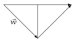
This is how the answer was given in the cited source. The vector triangle is as follows, so from the north west.
One.II.1.11 §II.1 source ↗
Euclid describes a plane as “a surface which lies evenly with the straight lines on itself”. Commentators such as Heron have interpreted this to mean, “(A plane surface is) such that, if a straight line pass through two points on it, the line coincides wholly with it at every spot, all ways”. (Translations from [Heath], pp. 171-172.) Do planes, as described in this section, have that property? Does this description adequately define planes?
Answer
Euclid no doubt is picturing a plane inside of . Observe, however, that both and also satisfy that definition.
One.II.2.11 §II.2 source ↗
Find the length of each vector.
Answer (5 parts)
One.II.2.12 §II.2 source ↗
Find the angle between each two, if it is defined.
Answer (3 parts)
Not defined.
One.II.2.13 §II.2 source ↗
[Ohanian] During maneuvers preceding the Battle of Jutland, the British battle cruiser Lion moved as follows (in nautical miles): miles north, miles degrees east of south, miles at degrees east of north, and miles at degrees east of north. Find the distance between starting and ending positions. (Ignore the earth’s curvature.)
Answer
We express each displacement as a vector, rounded to one decimal place because that’s the accuracy of the problem’s statement, and add to find the total displacement (ignoring the curvature of the earth).
The distance is .
One.II.2.14 §II.2 source ↗
Find so that these two vectors are perpendicular.
Answer
Solve to get .
One.II.2.15 §II.2 source ↗
Describe the set of vectors in orthogonal to the one with entries , , and .
Answer
We could describe the set
with parameters in this way.
One.II.2.16 §II.2 source ↗
Find the angle between the diagonal of the unit square in and any one of the axes.
Find the angle between the diagonal of the unit cube in and one of the axes.
Find the angle between the diagonal of the unit cube in and one of the axes.
What is the limit, as goes to , of the angle between the diagonal of the unit cube in and any one of the axes?
Answer (4 parts)
We can use the -axis.
Again, use the -axis.
The -axis worked before and it will work again.
Using the formula from the prior item, .
One.II.2.17 §II.2 source ↗
Is there any vector in that is perpendicular to itself?
Answer
Definition 2.7 stipulates that the angle between two vectors is a right angle if either is the zero vector. (It stipulates that separately since we cannot rely on the formula because the fraction’s denominator is .) Thus, by definition, the zero vector is perpendicular to itself.
It is the only such member of since is if and only if each is .
One.II.2.18 §II.2 source ↗
Describe the algebraic properties of dot product.
Is it right-distributive over addition: ?
Is it left-distributive (over addition)?
Does it commute?
Associate?
How does it interact with scalar multiplication?
As always, you must back any assertion with a suitable argument.
Answer (6 parts)
In each item below, assume that the vectors have components .
Dot product is right-distributive.
Dot product is also left distributive: . The proof is just like the prior one.
Dot product commutes.
Because is a scalar, not a vector, the expression makes no sense; the dot product of a scalar and a vector is not defined.
This is a vague question so it has many answers. Some are (1) and , (2) (in general; an example is easy to produce), and (3) (the connection between length and dot product is that the square of the length is the dot product of a vector with itself).
One.II.2.19 §II.2 source ↗
Verify the equality condition in Corollary 2.6, the Cauchy-Schwarz Inequality.
Show that if is a negative scalar multiple of then and are less than or equal to zero.
Show that if and only if one vector is a scalar multiple of the other.
Answer (2 parts)
Verifying that for and is easy. Now, for and , if then , which is times a nonnegative real.
The half is similar (actually, taking the in this paragraph to be the reciprocal of the above gives that we need only worry about the case).
We first consider the case. From the Triangle Inequality we know that if and only if one vector is a nonnegative scalar multiple of the other. But that’s all we need because the first part of this exercise shows that, in a context where the dot product of the two vectors is positive, the two statements ‘one vector is a scalar multiple of the other’ and ‘one vector is a nonnegative scalar multiple of the other’, are equivalent.
We finish by considering the case. Because and , we have that . Now the prior paragraph applies to give that one of the two vectors and is a scalar multiple of the other. But that’s equivalent to the assertion that one of the two vectors and is a scalar multiple of the other, as desired.
One.II.2.20 §II.2 source ↗
Suppose that and . Must ?
Answer
No. These give an example.
One.II.2.21 §II.2 source ↗
Does any vector have length zero except a zero vector? (If “yes”, produce an example. If “no”, prove it.)
Answer
We prove that a vector has length zero if and only if all its components are zero.
Let have components . Recall that the square of any real number is greater than or equal to zero, with equality only when that real is zero. Thus is a sum of numbers greater than or equal to zero, and so is itself greater than or equal to zero, with equality if and only if each is zero. Hence if and only if all the components of are zero.
One.II.2.22 §II.2 source ↗
Find the midpoint of the line segment connecting with in . Generalize to .
Answer
We can easily check that
is on the line connecting the two, and is equidistant from both. The generalization is obvious.
One.II.2.23 §II.2 source ↗
Show that if then has length one. What if ?
Answer
Assume that has components . If then we have this.
If then is not defined.
One.II.2.24 §II.2 source ↗
Show that if then is times as long as . What if ?
Answer
For the first question, assume that and , take the root, and factor.
For the second question, the result is times as long, but it points in the opposite direction in that .
One.II.2.25 §II.2 source ↗
A vector of length one is a unit vector. Show that the dot product of two unit vectors has absolute value less than or equal to one. Can ‘less than’ happen? Can ‘equal to’?
Answer
Assume that both have length . Apply Cauchy-Schwarz: .
To see that ‘less than’ can happen, in take
and note that . For ‘equal to’, note that .
One.II.2.26 §II.2 source ↗
When a plane does not pass through the origin, performing operations on vectors whose bodies lie in it is more complicated than when the plane does pass through the origin. Consider the picture in this subsection of the plane
and the three vectors with endpoints , , and .
Redraw the picture, including the vector starting at whose body is in the plane, and that is twice as long as the vector shown in the plane whose endpoint is . The endpoint of this vector is not ; what is it?
Redraw the picture, including the parallelogram in the plane that shows the sum of the vectors ending at and . The endpoint of the sum, on the diagonal, is not ; what is it?
Answer (2 parts)
The vector shown
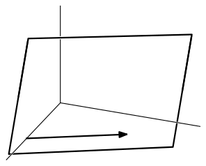
is not the result of doubling
instead it is the result of doubling the parameter.
This compares the lengths.
The vector
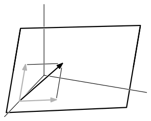
is not the result of adding
instead it is
which adds the parameters.
One.II.2.27 §II.2 source ↗
Show that the line segments and have the same lengths and slopes if and . Is that only if?
Answer
The “if” half is straightforward. If and then
so they have the same lengths, and the slopes are just as easy:
(if the denominators are they both have undefined slopes).
For “only if”, assume that the two segments have the same length and slope (the case of undefined slopes is easy; we will do the case where both segments have a slope ). Also assume, without loss of generality, that and that . The first segment is (for some intercept ) and the second segment is (for some ). Then the lengths of those segments are
and, similarly, . Therefore, . Thus, as we assumed that and , we have that .
The other equality is similar.
One.II.2.28 §II.2 source ↗
Is ? If it is true then it would generalize the Triangle Inequality.
Answer
Yes; we can prove this by induction.
Assume that the vectors are in some . Clearly the statement applies to one vector. The Triangle Inequality is this statement applied to two vectors. For an inductive step assume the statement is true for or fewer vectors. Then this
follows by the Triangle Inequality for two vectors. Now the inductive hypothesis, applied to the first summand on the right, gives that as less than or equal to .
One.II.2.29 §II.2 source ↗
What is the ratio between the sides in the Cauchy-Schwarz inequality?
Answer
By definition
where is the angle between the vectors. Thus the ratio is .
One.II.2.30 §II.2 source ↗
Describe the angle between two vectors in .
Answer
We can find the angle between and (for ) with
If or is zero then the angle is radians. Otherwise, if and are of opposite signs then the angle is radians, else the angle is zero radians.
One.II.2.31 §II.2 source ↗
Give a simple necessary and sufficient condition to determine whether the angle between two vectors is acute, right, or obtuse.
Answer
The angle between and is acute if , is right if , and is obtuse if . That’s because, in the formula for the angle, the denominator is never negative.
One.II.2.32 §II.2 source ↗
Generalize to the converse of the Pythagorean Theorem, that if and are perpendicular then .
Answer
Suppose that . If and are perpendicular then
(the third equality holds because ).
One.II.2.33 §II.2 source ↗
Show that if and only if and are perpendicular. Give an example in .
Answer
Where , the vectors and are perpendicular if and only if , which shows that those two are perpendicular if and only if . That holds if and only if .
One.II.2.34 §II.2 source ↗
Show that if a vector is perpendicular to each of two others then it is perpendicular to each vector in the plane they generate. (Remark. They could generate a degenerate plane — a line or a point — but the statement remains true.)
Answer
Suppose is perpendicular to both and . Then, for any we have this.
One.II.2.35 §II.2 source ↗
Prove that, where are nonzero vectors, the vector
bisects the angle between them. Illustrate in .
Answer
We will show something more general: if for , then bisects the angle between and
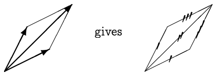
(we ignore the case where and are the zero vector).
The case is easy. For the rest, by the definition of angle, we will be finished if we show this.
But distributing inside each expression gives
and , so the two are equal.
One.II.2.36 §II.2 source ↗
Verify that the definition of angle is dimensionally correct: (1) if then the cosine of the angle between and equals the cosine of the angle between and , and (2) if then the cosine of the angle between and is the negative of the cosine of the angle between and .
Answer
We can show the two statements together. Let , write
and calculate.
One.II.2.37 §II.2 source ↗
Show that the inner product operation is linear: for and , .
Answer
Let
and then
as required.
One.II.2.38 §II.2 source ↗
[Cleary] Astrologers claim that they can recognize trends in personality and fortune that depend on an individual’s birthday by incorporating where the stars were centuries ago. Suppose that instead of star-gazers coming up with stuff, math teachers who like linear algebra (we’ll call them vectologers) had come up with a similar system as follows: Consider your birthday as a row vector . For instance, I was born on July so my vector would be . Vectologers assert that how well individuals get along with each other depends on the angle between vectors. The smaller the absolute value of that angle, the more harmonious the relationship.
Find the angle between your vector and mine, in radians.
Would you get along better with me, or with a professor born on September ?
For maximum harmony in a relationship, when should the other person be born?
Is there a person with whom you have a “worst case” relationship, i.e., your vector and theirs are orthogonal? If so, what are the birthdate(s) for such people? If not, explain why not.
Answer (4 parts)
My birthday of October gives this.
Applying the same equation to gives about radians.
The angle will measure radians if the other person is born on the same day. It will also measure if one birthday is a scalar multiple of the other. For instance, a person born on Mar would be harmonious with a person born on Feb .
Given a birthday, we can get Sage to plot the angle for other dates. This example shows the relationship of all dates with July 12.
  sage: plot3d(lambda x, y: math.acos((x*7+y*12)/(math.sqrt(7**2+12**2)*math.sqrt(x**2+y**2))),
                                                                 (1,12),(1,31))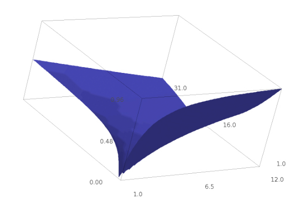
We want to maximize this.
Of course, we cannot take or negative and so we cannot get a vector orthogonal to the given one. This Python script finds the largest angle by brute force.
  import math
  days={1:31,  # Jan
        2:29, 3:31, 4:30, 5:31, 6:30, 7:31, 8:31, 9:30, 10:31, 11:30, 12:31}
  BDAY=(7,12)
  max_res=0
  max_res_date=(-1,-1)
  for month in range(1,13):
      for day in range(1,days[month]+1):
          num=BDAY[0]*month+BDAY[1]*day
          denom=math.sqrt(BDAY[0]**2+BDAY[1]**2)*math.sqrt(month**2+day**2)
          if denom>0:
              res=math.acos(min(num*1.0/denom,1))
              print "day:",str(month),str(day)," angle:",str(res)
              if res>max_res:
                  max_res=res
                  max_res_date=(month,day)
  print "For ",str(BDAY),"worst case",str(max_res),"rads, date",str(max_res_date)
  print "  That is ",180*max_res/math.pi,"degrees"
The result is
  For  (7, 12) worst case 0.95958064648 rads, date (12, 1)
    That is  54.9799211457 degrees
A more conceptual approach is to consider the relation of all points to the point . The picture below makes clear that the answer is either Dec or Jan , depending on which is further from the birthdate. The dashed line bisects the angle between the line from the origin to Dec , and the line from the origin to Jan . Birthdays above the line are furthest from Dec and birthdays below the line are furthest from Jan .
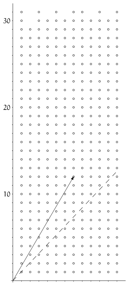
One.II.2.39 §II.2 source ↗
[Am. Math. Mon., Feb. 1933] A ship is sailing with speed and direction ; the wind blows apparently (judging by the vane on the mast) in the direction of a vector ; on changing the direction and speed of the ship from to the apparent wind is in the direction of a vector .
Find the vector velocity of the wind.
Answer
This is how the answer was given in the cited source. The actual velocity of the wind is the sum of the ship’s velocity and the apparent velocity of the wind. Without loss of generality we may assume and to be unit vectors, and may write
where and are undetermined scalars. Take the dot product first by and then by to obtain
Multiply the second by , subtract the result from the first, and find
Substituting in the original displayed equation, we get
One.II.2.40 §II.2 source ↗
Verify the Cauchy-Schwarz inequality by first proving Lagrange’s identity:
and then noting that the final term is positive. This result is an improvement over Cauchy-Schwarz because it gives a formula for the difference between the two sides. Interpret that difference in .
Answer
We use induction on .
In the base case the identity reduces to
and clearly holds.
For the inductive step assume that the formula holds for the , …, cases. We will show that it then holds in the case. Start with the right-hand side
and apply the inductive hypothesis.
to derive the left-hand side.
One.III.1.8 §III.1 source ↗
Use Gauss-Jordan reduction to solve each system.
Answer (5 parts)
These answers show only the Gauss-Jordan reduction. With it, describing the solution set is easy.
The solution set contains only a single element.
The solution set has one parameter.
There is a unique solution.
A row swap in the second step makes the arithmetic easier.
One.III.1.9 §III.1 source ↗
Do Gauss-Jordan reduction.
Answer (2 parts)
One.III.1.10 §III.1 source ↗
Find the reduced echelon form of each matrix.
Answer (5 parts)
Use Gauss-Jordan reduction.
The reduced echelon form is all zeroes except for a diagonal of ones.
As in the prior problem, the reduced echelon form is all zeroes but for a diagonal of ones.
There are more columns than rows so we must get more than just a diagonal of ones.
As in the prior item, this is not a square matrix.
One.III.1.11 §III.1 source ↗
Get the reduced echelon form of each.
Answer (2 parts)
Swap first.
Here the swap is in the middle.
One.III.1.12 §III.1 source ↗
Find each solution set by using Gauss-Jordan reduction and then reading off the parametrization.
Answer (5 parts)
For the Gauss’s halves, see the answers to Chapter One’s section I.2 question Exercise 2.19.
The “Jordan” half goes this way.
The solution set is this
The second half is
so the solution is this.
This Jordan half
gives
(of course, we could omit the zero vector from the description).
The “Jordan” half
ends with this solution set.
One.III.1.13 §III.1 source ↗
Give two distinct echelon form versions of this matrix.
Answer
Routine Gauss’s Method gives one:
and any cosmetic change, such as multiplying the bottom row by ,
gives another.
One.III.1.14 §III.1 source ↗
List the reduced echelon forms possible for each size.
Answer (5 parts)
In the cases listed below, we take . Thus, some canonical forms listed below actually include infinitely many cases. In particular, they includes the cases and .
, , ,
, , , , , ,
, , ,
, , , , , , ,
One.III.1.15 §III.1 source ↗
What results from applying Gauss-Jordan reduction to a nonsingular matrix?
Answer
A nonsingular homogeneous linear system has a unique solution. So a nonsingular matrix must reduce to a (square) matrix that is all ’s except for ’s down the upper-left to lower-right diagonal, such as these.
One.III.1.16 §III.1 source ↗
Decide whether each relation is an equivalence on the set of matrices.
two matrices are related if they have the same entry in the first row and first column
two matrices are related if they have the same entry in the first row and first column, or the same entry in the second row and second column
Answer (2 parts)
This is an equivalence.
We can write if they are related. The relation is reflexive because any matrix has the same entry as itself. The relation is symmetric because if has the same entry as then clearly also has the same entry as . Finally, the relation is transitive because if so they have the same entry as each other, and so they have the same as each other, then all three have the same entry, and .
This is not an equivalence because it is not transitive. The first and second matrix below are related by their entries, and the second and third are related by their entries. But the first and third are not related.
One.III.1.17 §III.1 source ↗
[Cleary] Consider the following relationship on the set of matrices: we say that is sum-what like if the sum of all of the entries in is the same as the sum of all the entries in . For instance, the zero matrix would be sum-what like the matrix whose first row had two sevens, and whose second row had two negative sevens. Prove or disprove that this is an equivalence relation on the set of matrices.
Answer
It is an equivalence relation. To prove that we must check that the relation is reflexive, symmetric, and transitive.
Assume that all matrices are . For reflexive, we note that a matrix has the same sum of entries as itself. For symmetric, we assume has the same sum of entries as and obviously then has the same sum of entries as . Transitivity is no harder — if has the same sum of entries as and has the same sum of entries as then has the same as .
One.III.1.18 §III.1 source ↗
The proof of Lemma 1.5 contains a reference to the condition on the row combination operation.
Write down a matrix with nonzero entries, and show that the operation is not reversed by .
Expand the proof of that lemma to make explicit exactly where it uses the condition on combining.
Answer (2 parts)
For instance,
leaves the matrix changed.
This operation
leaves the -th row unchanged because of the restriction. Because the -th row is unchanged, this operation
returns the -th row to its original state.
One.III.1.19 §III.1 source ↗
[Cleary] Consider the set of students in a class. Which of the following relationships are equivalence relations? Explain each answer in at least a sentence.
Two students are related if has taken at least as many math classes as .
Students are related if they have names that start with the same letter.
Answer (3 parts)
To be an equivalence, each relation must be reflexive, symmetric, and transitive.
This relation is not symmetric because if has taken classes and has taken then is related to but is not related to .
This is reflexive because ’s name starts with the same letter as does ’s. It is symmetric because if ’s name starts with the same letter as ’s then ’s starts with the same letter as does ’s. And it is transitive because if ’s name starts with the same letter as does ’s and ’s name starts with the same letter as does ’s then ’s starts with the same letter as does ’s. So it is an equivalence.
One.III.1.20 §III.1 source ↗
Show that each of these is an equivalence on the set of matrices. Describe the equivalence classes.
Two matrices are related if they have the same product down the diagonal, that is, if the product of the entries in the upper left and lower right are equal.
Two matrices are related if they both have at least one entry that is a , or if neither does.
Answer (3 parts)
For each we must check the three conditions of reflexivity, symmetry, and transitivity.
Any matrix clearly has the same product down the diagonal as itself, so the relation is reflexive. The relation is symmetric because if has the same product down its diagonal as does , if , then has the same product as does .
Transitivity is similar: suppose that ’s product is and that it equals ’s product. Suppose also that ’s product equals ’s. Then all three have a product of , and ’s equals ’s.
There is an equivalence class for each real number, namely the class contains all matrices whose product down the diagonal is that real.
For reflexivity, if the matrix has a entry then it is related to itself while if it does not then it is also related to itself. Symmetry also has two cases: suppose that and are related. If has a entry then so does , and thus is related to . If has no then neither does , and again is related to .
For transitivity, suppose that is related to and to . If has a entry then so does , and because is related to , therefore so does , and hence is related to . Likewise, if has no then neither does , and consequently neither does , giving the conclusion that is related to .
There are exactly two equivalence classes, one containing any matrix that has at least one entry that is a , and the other containing all the matrices that have no ’s.
One.III.1.21 §III.1 source ↗
Show that each is not an equivalence on the set of matrices.
Two matrices are related if .
Two matrices are related if the sum of their entries are within , that is, is related to if .
Answer (2 parts)
This relation is not reflexive. For instance, any matrix with an upper-left entry of is not related to itself.
This relation is not transitive. For these three, is related to , and is related to , but is not related to .
One.III.2.11 §III.2 source ↗
Decide if the matrices are row equivalent.
Answer (6 parts)
Bring each to reduced echelon form and compare.
The first gives
while the second gives
The two reduced echelon form matrices are not identical, and so the original matrices are not row equivalent.
The first is this.
The second is this.
These two are row equivalent.
These two are not row equivalent because they have different sizes.
The first,
and the second.
These are not row equivalent.
Here the first is
while this is the second.
These are not row equivalent.
One.III.2.12 §III.2 source ↗
Which of these matrices are row equivalent to each other?
Answer (7 parts)
Perform Gauss-Jordan reduction on each. Two matrices are row-equivalent if and only if they have the same reduced echelon form. Here is the reduced form for each.
One.III.2.13 §III.2 source ↗
Produce three other matrices row equivalent to the given one.
Answer (3 parts)
For each you can just perform some row operations on the starting matrix.
Multiplying the first row by gives this.
(There is no sense to this particular choice of row operation; it is just the first thing that came to mind.) Two other row operations are a row swap and adding .
Doing the same three arbitrary row operations gives these three.
One.III.2.14 §III.2 source ↗
Perform Gauss’s Method on this matrix. Express each row of the final matrix as a linear combination of the rows of the starting matrix.
Answer
The Gaussian reduction is routine.
Denoting those matrices , , and respectively, we have this.
One.III.2.15 §III.2 source ↗
Describe the matrices in each of the classes represented in Example 2.10.
Answer
First, the only matrix row equivalent to the matrix of all ’s is itself (since row operations have no effect).
Second, the matrices that reduce to
have the form
(where , and and are not both zero).
Next, the matrices that reduce to
have the form
(where , and not both are zero).
Finally, the matrices that reduce to
are the nonsingular matrices. That’s because a linear system for which this is the matrix of coefficients will have a unique solution, and that is the definition of nonsingular. (Another way to say the same thing is to say that they fall into none of the above classes.)
One.III.2.16 §III.2 source ↗
Describe all matrices in the row equivalence class of these.
Answer (3 parts)
They have the form
where at least one of is nonzero.
They have this form
where at least one of is nonzero.
The given matrix is nonsingular. So the row equivalence class consists of all nonsinglar matrices. (To give a formula, they have the form
for ) where . We will see in Chapter Four that this formula determines when a matrix is nonsingular.)
One.III.2.17 §III.2 source ↗
How many row equivalence classes are there?
Answer
Infinitely many. For instance, in
each gives a different class.
One.III.2.18 §III.2 source ↗
Can row equivalence classes contain different-sized matrices?
Answer
No. Row operations do not change the size of a matrix.
One.III.2.19 §III.2 source ↗
How big are the row equivalence classes?
Show that for any matrix of all zeros, the class is finite.
Do any other classes contain only finitely many members?
Answer (2 parts)
A row operation on a matrix of zeros has no effect. Thus each such matrix is alone in its row equivalence class.
No. Any nonzero entry can be rescaled.
One.III.2.20 §III.2 source ↗
Give two reduced echelon form matrices that have their leading entries in the same column but that are not row equivalent.
Answer
Here are two.
One.III.2.21 §III.2 source ↗
Show that any two nonsingular matrices are row equivalent. Are any two singular matrices row equivalent?
Answer
Any two nonsingular matrices have the same reduced echelon form, namely the matrix with all ’s except for ’s down the diagonal.
Two same-sized singular matrices need not be row equivalent. For example, these two singular matrices are not row equivalent.
One.III.2.22 §III.2 source ↗
Describe all of the row equivalence classes containing these.
matrices
matrices
matrices
matrices
Answer
Since there is one and only one reduced echelon form matrix in each class, we can just list the possible reduced echelon form matrices.
For that list, see the answer for Exercise 1.14.
One.III.2.23 §III.2 source ↗
Show that a vector is a linear combination of members of the set if and only if there is a linear relationship where is not zero. (Hint. Watch out for the case.)
Use that to simplify the proof of Lemma 2.5.
Answer (2 parts)
If there is a linear relationship where is not zero then we can subtract from both sides and divide by to get as a linear combination of the others. (Remark: if there are no other vectors in the set — if the relationship is, say, — then the statement is still true because the zero vector is by definition the sum of the empty set of vectors.)
Conversely, if is a combination of the others then subtracting from both sides gives a relationship where at least one of the coefficients is nonzero; namely, the in front of .
The first row is not a linear combination of the others for the reason given in the proof: in the equation of components from the column containing the leading entry of the first row, the only nonzero entry is the leading entry from the first row, so its coefficient must be zero. Thus, from the prior part of this exercise, the first row is in no linear relationship with the other rows.
Thus, when considering whether the second row can be in a linear relationship with the other rows, we can leave the first row out. But now the argument just applied to the first row will apply to the second row. (That is, we are arguing here by induction.)
One.III.2.24 §III.2 source ↗
[Trono] Three truck drivers went into a roadside cafe. One truck driver purchased four sandwiches, a cup of coffee, and ten doughnuts for $. Another driver purchased three sandwiches, a cup of coffee, and seven doughnuts for $. What did the third truck driver pay for a sandwich, a cup of coffee, and a doughnut?
Answer
We know that and that , and we’d like to know what is. Fortunately, is a linear combination of and . Calling the unknown price , we have this reduction.
The price paid is $.
One.III.2.25 §III.2 source ↗
The Linear Combination Lemma says which equations can be gotten from Gaussian reduction of a given linear system.
1. Produce an equation not implied by this system.
2. Can any equation be derived from an inconsistent system?
Answer
1. An easy answer is this.
For a less wiseguy-ish answer, solve the system:
gives and . Now any equation not satisfied by will do, e.g., .
2. Every equation can be derived from an inconsistent system. For instance, here is how to derive from . First,
(validity of the case is separate but clear). Similarly, . Ditto for . But now, gives .
One.III.2.26 §III.2 source ↗
[Hoffman & Kunze] Extend the definition of row equivalence to linear systems. Under your definition, do equivalent systems have the same solution set?
Answer
Define linear systems to be equivalent if their augmented matrices are row equivalent. The proof that equivalent systems have the same solution set is easy.
One.III.2.27 §III.2 source ↗
In this matrix
the first and second columns add to the third.
Show that remains true under any row operation.
Make a conjecture.
Prove that it holds.
Answer (3 parts)
The three possible row swaps are easy, as are the three possible rescalings. One of the six possible row combinations is :
and again the first and second columns add to the third. The other five combinations are similar.
The obvious conjecture is that row operations do not change linear relationships among columns.
A case-by-case proof follows the sketch given in the first item.
1 Topic: Computer Algebra Systems source ↗
Use the computer to solve the two problems that opened this chapter.
This is the Statics problem.
This is the Chemistry problem.
Answer (2 parts)
Sage does this.
sage: var('h,c')
(h, c)
sage: statics = [40*h + 15*c == 100,
....:            25*c == 50 + 50*h]
sage: solve(statics, h,c)
[[h == 1, c == 4]]
Other Computer Algebra Systems have similar commands. These Maple commands
> A:=array( [[40,15],
             [-50,25]] );
> u:=array([100,50]);
> linsolve(A,u);
get the answer [1,4].
Here there is a free variable. Sage gives this.
sage: var('h,i,j,k')
(h, i, j, k)
sage: chemistry = [7*h == 7*j,
....:              8*h + 1*i == 5*j + 2*k,
....:              1*i == 3*j,
....:              3*i == 6*j + 1*k]
sage: solve(chemistry, h,i,j,k)
[[h == 1/3*r1, i == r1, j == 1/3*r1, k == r1]]
Similarly, this Maple session
> A:=array( [[7,0,-7,0],
             [8,1,-5,2],
             [0,1,-3,0],
             [0,3,-6,-1]] );
> u:=array([0,0,0,0]);
> linsolve(A,u);
prompts the same reply (but with parameter ).
2 Topic: Computer Algebra Systems source ↗
Use the computer to solve these systems from the first subsection, or conclude ‘many solutions’ or ‘no solutions’.
Answer (6 parts)
The answer is and . A Sage session does this.
sage: var('x,y')
(x, y)
sage: system = [2*x + 2*y == 5,
....:              x - 4*y == 0]
sage: solve(system, x,y)
[[x == 2, y == (1/2)]]
A Maple session
> A:=array( [[2,2],
             [1,-4]] );
> u:=array([5,0]);
> linsolve(A,u);
gets the same answer, of course.
The answer is and .
sage: var('x,y')
(x, y)
sage: system = [-1*x + y == 1,
....:              x + y == 2]
sage: solve(system, x,y)
[[x == (1/2), y == (3/2)]]This system has infinitely many solutions. In the first subsection, with as a parameter, we got and . Sage gets the same.
sage: var('x,y,z')
(x, y, z)
sage: system = [x - 3*y + z == 1,
....:           x + y + 2*z == 14]
sage: solve(system, x,y)
[[x == -7/4*z + 43/4, y == -1/4*z + 13/4]]
Maple responds with , preferring as a parameter.
There is no solution to this system. Sage gives an empty list.
sage: var('x,y')
(x, y)
sage: system = [-1*x - y == 1,
....:           -3*x - 3*y == 2]
sage: solve(system, x,y)
[]
Similarly, When the array and vector are given to Maple and it is asked to linsolve(A,u), it returns no result at all; that is, it responds with no solutions.
Sage finds
sage: var('x,y,z')
(x, y, z)
sage: system = [       4*y + z == 20,
....:            2*x - 2*y + z == 0,
....:             x +        z == 5,
....:             x +    y - z == 10]
sage: solve(system, x,y,z)
[[x == 5, y == 5, z == 0]]
that the solutions is .
There are infinitely many solutions. Sage does this.
sage: var('x,y,z,w')
(x, y, z, w)
sage: system = [ 2*x +        z + w == 5,
....:                   y -       w == -1,
....:            3*x -        z - w == 0,
....:            4*x +  y + 2*z + w == 9]
sage: solve(system, x,y,z,w)
[[x == 1, y == r2 - 1, z == -r2 + 3, w == r2]]
Maple gives .
3 Topic: Computer Algebra Systems source ↗
Use the computer to solve these systems from the second subsection.
Answer (6 parts)
This system has infinitely many solutions. In the second subsection we gave the solution set as
and Sage finds
sage: var('x,y')
(x, y)
sage: system = [ 3*x + 6*y == 18,
....:              x + 2*y == 6]
sage: solve(system, x,y)
[[x == -2*r3 + 6, y == r3]]
while Maple responds with .
The solution set has only one member.
Sage gives this.
sage: var('x,y')
(x, y)
sage: system = [ x + y == 1,
....:            x - y == -1]
sage: solve(system, x,y)
[[x == 0, y == 1]]This system’s solution set is infinite
Sage gives this
sage: var('x1,x2,x3')
(x1, x2, x3)
sage: system = [   x1 +        x3 == 4,
....:              x1 - x2 + 2*x3 == 5,
....:            4*x1 - x2 + 5*x3 == 17]
sage: solve(system, x1,x2,x3)
[[x1 == -r4 + 4, x2 == r4 - 1, x3 == r4]]
and Maple gives .
There is a unique solution
and Sage finds it.
sage: var('a,b,c')
(a, b, c)
sage: system = [ 2*a +  b - c == 2,
....:            2*a +      c == 3,
....:              a - b      == 0]
sage: solve(system, a,b,c)
[[a == 1, b == 1, c == 1]]This system has infinitely many solutions; in the second subsection we described the solution set with two parameters.
Sage does the same.
sage: var('x,y,z,w')
(x, y, z, w)
sage: system = [   x + 2*y - z     == 3,
....:            2*x +   y     + w == 4,
....:              x -   y + z + w == 1]
sage: solve(system, x,y,z,w)
[[x == r6, y == -r5 - 2*r6 + 4, z == -2*r5 - 3*r6 + 5, w == r5]]
as does Maple .
The solution set is empty.
sage: var('x,y,z,w')
(x, y, z, w)
sage: system = [   x +      z + w == 4,
....:            2*x +  y     - w == 2,
....:            3*x +  y + z     == 7]
sage: solve(system, x,y,z,w)
[]
4 Topic: Computer Algebra Systems source ↗
What does the computer give for the solution of the general system?
Answer
Sage does this.
sage: var('x,y,a,b,c,d,p,q')
(x, y, a, b, c, d, p, q)
sage: system = [ a*x +  c*y == p,
....:            b*x +  d*y == q]
sage: solve(system, x,y)
[[x == -(d*p - c*q)/(b*c - a*d), y == (b*p - a*q)/(b*c - a*d)]]
In response to this prompting
> A:=array( [[a,c],
             [b,d]] );
> u:=array([p,q]);
> linsolve(A,u);
Maple gave this reply.
1 Topic: Input-Output Analysis source ↗
With the steel-auto system given above, estimate next year’s total productions in these cases.
Next year’s external demands are up from this year for steel and are unchanged for autos.
Next year’s external demands are up for steel and are up for autos.
Next year’s external demands are up for steel and are up for autos.
Answer (4 parts)
These answers are rounded to the number of decimal places given in the data, including when the data gives zero places.
Sage gets and .
sage: var('s,a')
(s, a)
sage: system = [(20053/25448)*s -  (2664/30346)*a == 17789,
....:             -(48/25448)*s + (21316/30346)*a == 21243]
sage: solve(system, s,a)
[[s == (2772443022712/106830469), a == (6476439541923/213660938)]]
sage: n(2772443022712/106830469), n(6476439541923/213660938)
(25951.8005365305, 30311.7621898814)Sage gets and .
sage: system = [(20053/25448)*s -  (2664/30346)*a == 17689,
....:             -(48/25448)*s + (21316/30346)*a == 21443]
sage: solve(system, s,a)
[[s == (2762271457112/106830469), a == (6537219545323/213660938)]]
sage: n(2762271457112/106830469), n(6537219545323/213660938)
(25856.5883213711, 30596.2316112410)Sage gets and .
sage: system = [(20053/25448)*s -  (2664/30346)*a == 17789,
....:             -(48/25448)*s + (21316/30346)*a == 21443]
sage: solve(system, s,a)
[[s == (2775832696312/106830469), a == (6537292375723/213660938)]]
sage: n(2775832696312/106830469), n(6537292375723/213660938)
(25983.5300012771, 30596.5724802865)
2 Topic: Input-Output Analysis source ↗
For the steel-auto system, with the external demand estimates of and discussed above, what will be the value of steel used by steel, the value of steel used by auto, etc.?
Answer
This Sage session
sage: var('a,s')
(a, s)
sage: eqns=[(20053/25448)*s - (2664/30346)*a == 17589,
....:       (-48/25448)*s + (21316/30346)*a == 21243]
sage: solve(eqns, s, a)
[[s == (2745320544312/106830469), a == (6476293881123/213660938)]]
sage: s_by_s = (5395/25448)*2745320544312/106830469
sage: s_by_s
582010544505/106830469
sage: n(s_by_s)
5447.98267716114
sage: s_by_a = (2664/30346)*6476293881123/213660938
sage: n(s_by_a)
2660.93449955743
sage: a_by_s = (48/25448)*2745320544312/106830469
sage: n(a_by_s)
48.4713936058822
sage: a_by_a = (9030/30346)*6476293881123/213660938
sage: n(a_by_a)
9019.60905818451
gives this table.
|
|
| total | |||||||
| ||||||||||
|
For comparison here is the original table.
|
|
| total | |||||||
| ||||||||||
|
3 Topic: Input-Output Analysis source ↗
In the steel-auto system, the ratio for the use of steel by the auto industry is , about . Imagine that a new process for making autos reduces this ratio to .
How will the predictions for next year’s total productions change compared to the first example discussed above, that is, where next year’s external demands are for steel and for autos?
Predict next year’s totals if in addition, the external demand for autos rises to be because the new process makes cars cheaper.
Answer (2 parts)
Sage gives , .
 sage: var('s,a')
(s, a)
sage: system = [(20053/25448)*s -  0.0500*a == 17589,
....:             -(48/25448)*s + (21316/30346)*a == 21243]
sage: solve(system, s,a)
[[s == (12951731858499/534221147), a == (32381469405615/1068442294)]]
sage: n(12951731858499/534221147), n(32381469405615/1068442294)
(24244.1392131918, 30307.1767071166)Sage gives , .
sage: system = [(20053/25448)*s -  0.0500*a == 17589,
....:             -(48/25448)*s + (21316/30346)*a == 21500]
sage: solve(system, s,a)
[[s == (12964136043940/534221147), a == (16386224431390/534221147)]]
sage: n(12964136043940/534221147), n(16386224431390/534221147)
(24267.3584090448, 30673.1107957993)
4 Topic: Input-Output Analysis source ↗
This table gives the numbers for the auto-steel system from a different year, 1947 (see [Leontief 1951]). The units here are billions of 1947 dollars.
|
|
| total | |||||||
| ||||||||||
|
Solve for total output if next year’s external demands are: steel’s demand up % and auto’s demand up %.
How do the ratios compare to those given above in the discussion for the 1958 economy?
Illustrate the effect of how the ratios change over time by using the 1947 ratios from the first item with the 1958 external demands. Compare the predictions for total output. (Inflation was between the two years, but note that inflation does not affect the ‘’ ratios because the factor of is in both the numerator and the denominator.)
Answer (3 parts)
These are the equations, where the units are 1958 billions.
Sage gives this result (including an inital check).
sage: var('a,s')
(a, s)
sage: eqns=[(11.79/18.69)*s - (1.28/14.27)*a == 10.51,
....:       (-0)*s         + (9.87/14.27)*a == 9.87]
sage: solve(eqns,s,a)
[[s == (1869/100), a == (1427/100)]]
sage: n(1869/100)
18.6900000000000
sage: n(1427/100)
14.2700000000000
sage: eqns=[(11.79/18.69)*s - (1.28/14.27)*a == 11.561,
....:       (-0)*s         + (9.87/14.27)*a == 11.3505]
sage: solve(eqns,s,a)
[[s == (8119559/393000), a == (32821/2000)]]
sage: n(8119559/393000)
20.6604554707379
sage: n(32821/2000)
16.4105000000000These are the 1947 ratios, to three decimal places.
| 1947 | by steel | by autos |
| use of steel | ||
| use of autos |
These are the 1958 ratios.
| 1958 | by steel | by autos |
| use of steel | ||
| use of autos |
The external demands in 1958 are and , in billions of 1958 dollars. In 1948 dollars those are and . Sage gives these numbers.
sage: eqns=[(11.79/18.69)*s - (1.28/14.27)*a == 13.53,
....:       (-0)*s         + (9.87/14.27)*a == 16.34]
sage: solve(eqns,s,a)
[[s == (137466107/5541300), a == (1165859/49350)]]
sage: n(137466107/5541300)
24.8075554472777
sage: n(1165859/49350)
23.6242958459980
Converting back to 1958 dollars by multiplying by gives and .
5 Topic: Input-Output Analysis source ↗
Predict next year’s total productions of each of the three sectors of the hypothetical economy shown below
|
|
|
| total | |||||||||
| |||||||||||||
| |||||||||||||
|
if next year’s external demands are as stated.
for farm, for rail, for shipping
for farm, for rail, for shipping
Answer (2 parts)
These commands in Sage
var('f, r, s')
farm_by_farm = 25
farm_by_rail = 50
farm_by_ship = 100
farm_total = 800
# farm_by_others = farm_total -farm_by_farm - farm_by_rail - farm_by_ship
rail_by_farm = 25
rail_by_rail = 50
rail_by_ship = 50
rail_total = 300
# rail_by_others = rail_total -rail_by_farm - rail_by_rail - rail_by_ship
ship_by_farm = 15
ship_by_rail = 10
ship_by_ship = 0
ship_total = 500
# ship_by_others = ship_total - ship_by_farm - ship_by_rail - ship_by_ship

farm_by_others = 625
rail_by_others = 200
ship_by_others = 475
sys = [(farm_by_farm/farm_total)*f + (farm_by_rail/rail_total)*r + (farm_by_ship/ship_total)*s + farm_by_others == f,
(rail_by_farm/farm_total)*f + (rail_by_rail/rail_total)*r + (rail_by_ship/ship_total)*s + rail_by_others == r,
(ship_by_farm/farm_total)*f + (ship_by_rail/rail_total)*r + (ship_by_ship/ship_total)*s + ship_by_others == s ]
sols = solve(sys, f, r, s, solution_dict=True)
farm = sols[0][f]
rail = sols[0][r]
ship = sols[0][s]
give the conclusion that , , and .
Changing the lines in the prior item to these.
farm_by_others = 650
rail_by_others = 150
ship_by_others = 450
gives the solution , , and .
6 Topic: Input-Output Analysis source ↗
This table gives the interrelationships among three segments of an economy (see [Clark & Coupe]).
|
|
|
| total | |||||||||
| |||||||||||||
| |||||||||||||
|
We will do an Input-Output analysis on this system.
Fill in the numbers for this year’s external demands.
Solve the system where we get next year’s external demands by taking this year’s external demands and inflating them %. Do all three sector totals increase by %? Do they even increase at the same rate?
Solve the system where we get next year’s external demands by taking this year’s external demands and reducing them %. (The study source for these numbers concluded that because of the closing of a local military facility, overall personal income in the area would fall %, so this might be a first guess at what would happen.)
Answer (4 parts)
This is the basic setup in Sage.
var('f, w, r')
food_by_food = 0
food_by_whole = 2318
food_by_retail = 4679
food_total = 11869
food_by_others = food_total - food_by_food - food_by_whole - food_by_retail
whole_by_food = 393
whole_by_whole = 1089
whole_by_retail = 22459
whole_total = 122242
whole_by_others = whole_total - whole_by_food - whole_by_whole - whole_by_retail
retail_by_food = 3
retail_by_whole = 53
retail_by_retail = 75
retail_total = 116041
retail_by_others = retail_total - retail_by_food - retail_by_whole - retail_by_retail

sys = [(food_by_food/food_total)*f + (food_by_whole/whole_total)*w + (food_by_retail/retail_total)*r + food_by_others == f,
(whole_by_food/food_total)*f + (whole_by_whole/whole_total)*w + (whole_by_retail/retail_total)*r + whole_by_others == w,
(retail_by_food/food_total)*f + (retail_by_whole/whole_total)*w + (retail_by_retail/retail_total)*r + retail_by_others == r ]
sols = solve(sys, f, w, r, solution_dict=True)
food = sols[0][f]
whole = sols[0][w]
retail = sols[0][r]With that, Sage gives that external food is , external wholesale is , and external retail is .
With ten percent inflation in the external demand numbers, the solutions are , , and .
The seven percent deflation in external demand gives , , and .
1 Topic: Accuracy of Computations source ↗
Using two decimal place numbers, add and .
Answer
Scientific notation is convenient for expressing the two-place restriction: . Adding the has no effect.
2 Topic: Accuracy of Computations source ↗
Solve this system (from [Rice]) by rounding at each step to four digits.
Answer
Reduction uses the step . First, and rounding to four digits gives . We take that the leading entry in the second row is now zero (that’s the point of the row reduction step). For the second entry, , which rounds to four digits as . Adding rounds to . As to the third entry, rounds to , and adding rounds to .
The conclusion is that is , which rounds to . Substituting gives , which rounds to , and then rounds to . Solving gives , which is . Checking that by substitution into the original equations shows that it is correct.
3 Topic: Accuracy of Computations source ↗
Assume that the machine uses four digit numbers.
Show that it will compute as unequal to when , and , and .
Compare the computer’s versions of and . Is twice the first equation the same as the second?
Answer (2 parts)
For the first, is zero and so is . For the other, is rounded to four digits, . Then is zero.
The first equation is while the second is . Twice the first is , so they aren’t equal.
4 Topic: Accuracy of Computations source ↗
Ill-conditioning is not only dependent on the matrix of coefficients. This example [Hamming] shows that it can arise from an interaction between the left and right sides of the system. Let be a small real.
Solve the system by hand. Notice that the ’s divide out only because there is an exact cancellation of the integer parts on the right side as well as on the left.
Solve the system by hand, rounding to two decimal places, and with .
Answer (2 parts)
Here is the calculation.
The third equation is . Cancel the ’s and solve to get . Substitute into the second equation.
Thus and so . Then the first equation says that .
As above, scientific notation is convenient to express the restriction on the number of digits. With two digits
we get , , and . These differ significantly from the true values found in the first part.
1 Topic: Analyzing Networks source ↗
Calculate the amperages in each part of each network.
This is a simple network.
Compare this one with the parallel case discussed above.
This is a reasonably complicated network.
Answer (3 parts)
The total resistance is ohms. With a volt potential, the flow will be amperes. The voltage drops will then be: volts across the ohm resistor, and volts across each of the two ohm resistors.
The ohm resistor on the left has a voltage drop of volts (and hence the flow through it is amperes), and the remaining portion on the right also has a voltage drop of volts, and so we can analyze it as in the prior item. We can also use linear systems.
The Current Law applied to junction in the the upper middle gives . Applied to the lower middle junction it gives . The Voltage Law applied to the leftmost circuit is that the volts up equals the voltage drop across the ohm resistor, . The rightmost circuit has a total resistance of ohm, so the Voltage Law gives . Here is the linear system.
Gauss’s Method
gives the unique solution , , , and .
Using these variables,
below is one linear system sufficient to yield the solution. The first four equations are from the Current Law. The last three are from applying the Voltage Law to the circuit involving --, the circuit involving ----, and the circuit with ----.
Gauss’s Method gives , , , , , , and .
2 Topic: Analyzing Networks source ↗
In the first network that we analyzed, with the three resistors in series, we just added to get that they acted together like a single resistor of ohms. We can do a similar thing for parallel circuits. In the second circuit analyzed,
we found that the current through the battery is amperes. Thus, the parallel portion is equivalent to a single resistor of ohms.
What is the equivalent resistance if we change the ohm resistor to ohms?
What is the equivalent resistance if the two are each ohms?
Find the formula for the equivalent resistance if the two resistors in parallel are ohms and ohms.
Answer (3 parts)
Using the variables from the earlier analysis,
Gauss’s Method gives that the current flowing in each branch is , , and , all in amperes. Thus the parallel portion is acting as a single resistor of ohms.
A similar analysis
gives that , , and amperes. The equivalent resistance is ohms.
Another analysis like the prior ones
gives , , and , all in amperes. The parallel portion is acting as a single resistor of size ohms. (This equation is often stated as: the equivalent resistance satisfies .)
3 Topic: Analyzing Networks source ↗
A Wheatstone bridge is used to measure resistance.
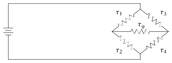
Show that in this circuit if the current flowing through is zero then . (To operate the device, put the unknown resistance at . At is a meter that shows the current. We vary the three resistances , , and — typically they each have a calibrated knob — until the current in the middle reads . Then the equation gives the value of .)
Answer
Kirchoff’s Current Law, applied to the node where , , and come together, and also applied to the node where , , and come together gives these.
Kirchoff’s Voltage law, applied to the loop in the top right, and to the loop in the bottom right, gives these.
Assuming that is zero gives that , that , that , and that . Then rearranging the last equality
and cancelling the ’s gives the desired conclusion.
4 Topic: Analyzing Networks source ↗
Consider this traffic circle.
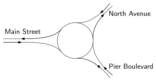
This is the traffic volume, in units of cars per ten minutes.
| North | Pier | Main | |||||||||
|
We can set up equations to model how the traffic flows.
Adapt Kirchhoff’s Current Law to this circumstance. Is it a reasonable modeling assumption?
Label the three between-road arcs in the circle with a variable: let be the number of cars going from North Avenue to Main, let be the number of cars between Main and Pier, and let be the number between Pier and North. Using the adapted law, for each of the three in-out intersections state an equation describing the traffic flow at that node.
Solve that system.
Interpret your solution.
Restate the Voltage Law for this circumstance. How reasonable is it?
Answer (5 parts)
An adaptation is: in any intersection the flow in equals the flow out. It does seem reasonable in this case, unless cars are stuck at an intersection for a long time.
Because cars leave via Main while cars enter, . Similarly Pier’s in/out balance means that and North gives . We have this system.
The row operations and lead to the conclusion that there are infinitely many solutions. With as the parameter, this is the solution set.
Since the problem is stated in number of cars we might restrict to be a natural number.
If we picture an initially-empty circle with the given input/output behavior, we can superimpose -many cars circling endlessly to get a new solution.
A suitable restatement might be: the number of cars entering the circle must equal the number of cars leaving. The reasonableness of this one is not as clear. Over the five minute time period we could find that a half dozen more cars entered than left, although the problem statement’s into/out table does satisfy this property. In any event, it is of no help in getting a unique solution since for that we would need to know the number of cars circling endlessly.
5 Topic: Analyzing Networks source ↗
This is a network of streets.
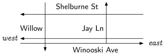
We can observe the hourly flow of cars into this network’s entrances, and out of its exits.
| east Winooski | west Winooski | Willow | Jay | Shelburne | |||||||||||||
|
|
(Note that to reach Jay a car must enter the network via some other road first, which is why there is no ‘into Jay’ entry in the table. Note also that over a long period of time, the total in must approximately equal the total out, which is why both rows add to cars.) Once inside the network, the traffic may flow in different ways, perhaps filling Willow and leaving Jay mostly empty, or perhaps flowing in some other way. Kirchhoff’s Laws give the limits on that freedom.
Determine the restrictions on the flow inside this network of streets by setting up a variable for each block, establishing the equations, and solving them. Notice that some streets are one-way only. (Hint: this will not yield a unique solution, since traffic can flow through this network in various ways; you should get at least one free variable.)
Suppose that someone proposes construction for Winooski Avenue East between Willow and Jay, and traffic on that block will be reduced. What is the least amount of traffic flow that can we can allow on that block without disrupting the hourly flow into and out of the network?
Answer (2 parts)
Here is a variable for each unknown block; each known block has the flow shown.
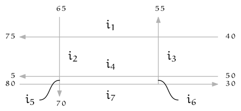
We apply Kirchhoff’s principle that the flow into the intersection of Willow and Shelburne must equal the flow out to get . Doing the intersections from right to left and top to bottom gives these equations.
The row operation followed by then and and finally result in this system.
Since the free variables are and we take them as parameters.
Obviously and have to be positive, and in fact the first equation shows that must be at least . If we start with , then the equation shows that .
We cannot take to be zero or else will be negative (this would mean cars going the wrong way on the one-way street Jay). We can, however, take to be as small as , and then there are many suitable ’s. For instance, the solution
results from choosing .
Loading chapter 2…
Exercises and answers are adapted from Linear Algebra by Jim Hefferon, which is free to read and download, and are used under the CC BY-SA 2.5 licence. They are taken from the book’s LaTeX source and set for the web, so they may differ slightly from the printed page. This adaptation is released under the same licence and is neither affiliated with nor endorsed by Jim Hefferon.