Every problem in the chapter beside the book’s answer, a chapter at a time as you scroll.
Chapter 5: Similarity
166 problems · 2 figuresFive.II.1.5 §II.1 source ↗
For
check that .
Answer
One way to proceed is left to right.
Five.II.1.6 §II.1 source ↗
Example 1.4 shows that the only matrix similar to a zero matrix is itself and that the only matrix similar to the identity is itself.
Show that the matrix whose single entry is is also similar only to itself.
Is a matrix of the form for some scalar similar only to itself?
Is a diagonal matrix similar only to itself?
Answer (3 parts)
Because the matrix is , the matrices and are also and so where the inverse is . Thus .
Yes: recall that we can bring scalar multiples out of a matrix . By the way, the zero and identity matrices are the special cases and .
No, as this example shows.
Five.II.1.7 §II.1 source ↗
Consider this transformation of
and these bases.
We will compute the parts of the arrow diagram to represent the transformation using two similar matrices.
Draw the arrow diagram, specialized for this case.
Compute .
Compute .
Compute the matrices for the other two sides of the arrow square.
Answer (4 parts)
For each element of the starting basis find the effect of the transformation
and represented those outputs with respect to the ending basis
to get the matrix.
Find the effect of the transformation on the elements of
and represented those with respect to the ending basis
to get the matrix.
To go down on the right we need so we first compute the effect of the identity map on each element of , which is no effect, and then represent the results with respect to .
So this is .
For the other matrix we can either find it directly, as we just have with , or we can do the usual calculation of a matrix inverse.
Five.II.1.8 §II.1 source ↗
Consider the transformation described by , , and .
Find where .
Find where .
Find the matrix such that .
Answer (3 parts)
Because we describe with the members of , finding the matrix representation is easy:
gives this.
We will find , , and , to find how each is represented with respect to . We are given that , and the other two are easy to see: and . By eye, we get the representation of each vector
and thus the representation of the map.
The diagram
shows that these are and .
Five.II.1.9 §II.1 source ↗
Let represent with respect to .
We will convert to the matrix representing with respect to .
Draw the arrow diagram.
Give the matrix that represents the left and right sides of that diagram, in the direction that we traverse the diagram to make the conversion.
Find .
Answer (3 parts)
For the right side we find the effect of the identity map, which is no effect,
and represent those with respect to
so we have this.
For the matrix on the left we can either compute it directly, as in the prior paragraph, or we can take the inverse.
As with the prior item we can either compute it directly from the definition or compute it using matrix operations.
Five.II.1.10 §II.1 source ↗
Exhibit a nontrivial similarity relationship by letting act in this way,
picking two bases , and representing with respect to them, and . Then compute the and to change bases from to and back again.
Answer
One possible choice of the bases is
(this comes from the map description). To find the matrix , solve the relations
to get , , and .
Finding involves a bit more computation. We first find . The relation
gives and , and so
making
and hence acts on the first basis vector in this way.
The computation for is similar. The relation
gives and , so
making
and hence acts on the second basis vector in this way.
Therefore
and so this matrix.
and this one change the bases.
The check of these computations is routine.
Five.II.1.11 §II.1 source ↗
Show that these matrices are not similar.
Answer
Gauss’s Method shows that the first matrix represents maps of rank two while the second matrix represents maps of rank three.
Five.II.1.12 §II.1 source ↗
Explain Example 1.4 in terms of maps.
Answer
The only representation of a zero map is a zero matrix, no matter what the pair of bases , and so in particular for any single basis we have . The case of the identity is slightly different: the only representation of the identity map, with respect to any , is the identity . (Remark: of course, we have seen examples where and — in fact, we have seen that any nonsingular matrix is a representation of the identity map with respect to some .)
Five.II.1.13 §II.1 source ↗
[Halmos] Are there two matrices and that are similar while and are not similar?
Answer
No. If then .
Five.II.1.14 §II.1 source ↗
Prove that if two matrices are similar and one is invertible then so is the other.
Answer
Matrix similarity is a special case of matrix equivalence (if matrices are similar then they are matrix equivalent) and matrix equivalence preserves nonsingularity.
Five.II.1.15 §II.1 source ↗
Show that similarity is an equivalence relation. (The definition given earlier already reflects this, so instead start here with the definition that is similar to if .)
Answer
A matrix is similar to itself; take to be the identity matrix: .
If is similar to then and so . Rewrite to conclude that is similar to .
For transitivity, if is similar to and is similar to then and . Then , showing that is similar to .
Five.II.1.16 §II.1 source ↗
Consider a matrix representing, with respect to some , reflection across the -axis in . Consider also a matrix representing, with respect to some , reflection across the -axis. Must they be similar?
Answer
Let and be the reflection maps (sometimes called ‘flip’s). For any bases and , the matrices and are similar. First note that
are similar because the second matrix is the representation of with respect to the basis :
where .
Now the conclusion follows from the transitivity part of Exercise 1.15.
We can also finish without relying on that exercise. Write and . By the equation in the first paragraph, the first of these two is . Rewriting the second of these two as and substituting gives the desired relationship
Thus the matrices and are similar.
Five.II.1.17 §II.1 source ↗
Prove that matrix similarity preserves rank and determinant. Does the converse hold?
Answer
We must show that if two matrices are similar then they have the same rank and the same determinant.
First, we’ve shown that the rank of a map equals the rank of any matrix representing that map, so the rank must be the same for all representations. (Said another way, rank is a property of the map since it is the dimension of the range space.)
As for determinants, .
The converse of the statement does not hold. For one thing, there are matrices with the same determinant that are not similar. As an example, consider a nonzero matrix with a determinant of zero. It is not similar to the zero matrix because the zero matrix is similar only to itself, but they have they same determinant. The same thinking gives an example for rank.
Five.II.1.18 §II.1 source ↗
Is there a matrix equivalence class with only one matrix similarity class inside? One with infinitely many similarity classes?
Answer
The matrix equivalence class containing all rank zero matrices contains only a single matrix, the zero matrix. Therefore it has as a subset only one similarity class.
In contrast, the matrix equivalence class of matrices of rank one consists of those matrices where . For any basis , the representation of multiplication by the scalar is , so each such matrix is alone in its similarity class. So this is a case where a matrix equivalence class splits into infinitely many similarity classes.
Five.II.1.19 §II.1 source ↗
Can two different diagonal matrices be in the same similarity class?
Answer
Yes, these are similar
since, where the first matrix is for , the second matrix is for .
Five.II.1.20 §II.1 source ↗
Prove that if two matrices are similar then their -th powers are similar when . What if ?
Answer
The -th powers are similar because, where each matrix represents the map , the -th powers represent , the composition of -many ’s. (For instance, if then .)
Restated more computationally, if then . Induction extends that to all powers.
For the case, suppose that is invertible and that . Note that is invertible: , and that same equation shows that is similar to . Other negative powers are now given by the first paragraph.
Five.II.1.21 §II.1 source ↗
Let be the polynomial . Show that if is similar to then is similar to .
Answer
In conceptual terms, both represent for some transformation . In computational terms, we have this.
Five.II.1.22 §II.1 source ↗
List all of the matrix equivalence classes of matrices. Also list the similarity classes, and describe which similarity classes are contained inside of each matrix equivalence class.
Answer
There are two equivalence classes, (i) the class of rank zero matrices, of which there is one: , and (2) the class of rank one matrices, of which there are infinitely many: .
Each matrix is alone in its similarity class. That’s because any transformation of a one-dimensional space is multiplication by a scalar given by . Thus, for any basis , the matrix representing a transformation with respect to is .
So, contained in the matrix equivalence class is (obviously) the single similarity class consisting of the matrix . And, contained in the matrix equivalence class are the infinitely many, one-member-each, similarity classes consisting of for .
Five.II.1.23 §II.1 source ↗
Does similarity preserve sums?
Answer
No. Here is an example that has two pairs, each of two similar matrices:
and
(this example is not entirely arbitrary because the center matrices on the two left sides add to the zero matrix). Note that the sums of these similar matrices are not similar
since the zero matrix is similar only to itself.
Five.II.1.24 §II.1 source ↗
Show that if and are similar matrices then and are also similar.
Answer
If then . The diagonal matrix commutes with anything, so . Thus and consequently . (So not only are they similar, in fact they are similar via the same .)
Five.II.2.6 §II.2 source ↗
Repeat Example 2.5 for the matrix from Example 2.2.
Answer
Because we chose the basis vectors arbitrarily, many different answers are possible. However, here is one way to go; to diagonalize
take it as the representation of a transformation with respect to the standard basis and look for such that
that is, such that and .
We are looking for scalars such that this equation
has solutions and , which are not both zero. Rewrite that as a linear system
If then the first equation gives that , and then the second equation gives that . We have disallowed the case where both ’s are zero so we can assume that .
Consider the bottom equation. If then the first equation gives or . The case is not allowed. The other possibility for the bottom equation is that the numerator of the fraction is zero. The case gives a first equation of , and so associated with we have vectors whose first and second components are equal:
If then the first equation is and so the associated vectors are those whose first component is twice their second:
This picture
shows how to get the diagonalization.
Comment. This equation matches the definition under this renaming.
Five.II.2.7 §II.2 source ↗
Diagonalize this matrix by following the steps of Example 2.5.
Set up the matrix-vector equation described in Lemma 2.4 and rewrite it as a linear system.
By considering solutions for that system, find two vectors to make a basis. (Consider separately the system in the and cases. Also, recall that the zero vector cannot be a member of a basis.)
Use that basis in the similarity diagram to get the diagonal matrix as the product of three others.
Answer (3 parts)
We want a basis where the member vectors satisfy
so consider the resulting linear system.
If then , so . That is, associated with this case are basis elements where the entries have opposite signs. (The entries must be nonzero since the zero vector cannot be a member of a basis.)
If then and substituting that into the top equation gives . So in this case, either or . But since in this case, is impossible because the zero vector is not in any basis. Thus and the system becomes this.
So this case is associated with basis elements where and can have any nonzero value.
Therefore, a suitable basis is this.
With that basis, to get the diagonalization, draw the similarity diagram.
In this diagram,
and we will calculate the matrix using the basis and traversing the lower-left to upper-left, to upper-right, and to lower-right path.
We first want to go from the lower-left to the upper-left. Observe that because we have chosen the basis for the top of the diagram to be the standard basis , the matrix representing that map is easy.
The calculation for the entire path does indeed give a diagonal result (of course, the lower-left to upper-left portion appears on the right side of the product of the three matrices).
Five.II.2.8 §II.2 source ↗
Follow Example 2.5 to diagonalize this matrix.
Set up the matrix-vector equation and rewrite it as a linear system.
By considering solutions for that system, find two vectors to make a basis. (Consider separately the and cases. Also, recall that the zero vector cannot be a member of a basis.)
With that basis use the similarity diagram to get the diagonalization as the product of three matrices.
Answer (3 parts)
The members of the basis satisfy this.
so this is the resulting linear system.
If then , but the zero vector is not a member of any basis so this case cannot happen.
The other case is .
Focus on the bottom equation. Either or . If then substituting into the top equation gives since is the assumption of this case. But the zero vector is not a member of any basis so this cannot happen.
We are left with this.
If then the system is
and so basis vectors satisfy . If then the system is
and basis vectors satisfy . Therefore, this is an example of a suitable basis.
To get the diagonalization, draw the similarity diagram
where is the matrix give in the problem statement.
Calculate the matrix using the basis by moving from the lower left to the upper left, to the upper right, and then to the lower right.
Observe that the matrix representing the lower left to upper left map is easy.
With that, the calculation for the entire path does give a diagonal result.
Five.II.2.9 §II.2 source ↗
Diagonalize these upper triangular matrices.
Answer (2 parts)
Setting up
gives the two possibilities that and . Following the possibility leads to the first equation with the two cases that and that . Thus, under this first possibility, we find and the associated vectors whose second component is zero, and whose first component is free.
Following the other possibility leads to a first equation of and so the vectors associated with this solution have a second component that is four times their first component.
The diagonalization is this.
The calculations are like those in the prior part.
The bottom equation gives the two possibilities that and . Following the possibility, and discarding the case where both and are zero, gives that , associated with vectors whose second component is zero and whose first component is free.
The possibility gives a first equation of and so the associated vectors have a second component that is the negative of their first component.
We thus have this diagonalization.
Five.II.2.10 §II.2 source ↗
If we try to diagonalize the matrix of Example 2.3
using the method of Example 2.5 then what goes wrong?
Draw the similarity diagram with .
Set up the matrix-vector equation described in Lemma 2.4 and rewrite it as a linear system.
By considering solutions for that system, find the trouble. (Consider separately the and cases.)
Answer (2 parts)
In this similarity diagram
we will try to calculate the matrix and find a suitable basis , by traversing the lower-left to upper-left, to upper-right, and to lower-right path.
The diagram shows that where we want and . To determine and , where the matrix represents the map with respect to the standard bases, we want to find solutions of this system.
The equivalent linear system
By the first line, either or . If then the second equation becomes so and we get this solution set.
We can take the initial member of the basis to be .
If then the first equation of the linear system gives . The system’s first line becomes and its second line becomes . Since this case takes , we get and the set of solutions is trivial.
So what goes wrong is that we don’t get the basis required by Lemma 2.4.
Five.II.2.11 §II.2 source ↗
What form do the powers of a diagonal matrix have?
Answer
For any integer , we have this.
Five.II.2.12 §II.2 source ↗
Give two same-sized diagonal matrices that are not similar. Must any two different diagonal matrices come from different similarity classes?
Answer
These two are not similar
because each is alone in its similarity class.
For the second half, these
are similar via the matrix that changes bases from to . (Question. Are two diagonal matrices similar if and only if their diagonal entries are permutations of each others?)
Five.II.2.13 §II.2 source ↗
Give a nonsingular diagonal matrix. Can a diagonal matrix ever be singular?
Answer
Contrast these two.
The first is nonsingular, the second is singular.
Five.II.2.14 §II.2 source ↗
Show that the inverse of a diagonal matrix is the diagonal of the inverses, if no element on that diagonal is zero. What happens when a diagonal entry is zero?
Answer
To check that the inverse of a diagonal matrix is the diagonal matrix of the inverses, just multiply.
(Showing that it is a left inverse is just as easy.)
If a diagonal entry is zero then the diagonal matrix is singular; it has a zero determinant.
Five.II.2.15 §II.2 source ↗
The equation ending Example 2.5
is a bit jarring because for we must take the first matrix, which is shown as an inverse, and for we take the inverse of the first matrix, so that the two powers cancel and this matrix is shown without a superscript .
Check that this nicer-appearing equation holds.
Is the previous item a coincidence? Or can we always switch the and the ?
Answer (2 parts)
The check is easy.
It is a coincidence, in the sense that if then need not equal . Even in the case of a diagonal matrix , the condition that does not imply that equals . The matrices from Example 2.2 show this.
Five.II.2.16 §II.2 source ↗
Show that the used to diagonalize in Example 2.5 is not unique.
Answer
The columns of the matrix are the vectors associated with the ’s. The exact choice, and the order of the choice was arbitrary. We could, for instance, get a different matrix by swapping the two columns.
Five.II.2.17 §II.2 source ↗
Find a formula for the powers of this matrix. Hint: see Exercise 2.11.
Answer
Diagonalizing and then taking powers of the diagonal matrix shows that
Five.II.2.18 §II.2 source ↗
We can ask how diagonalization interacts with the matrix operations. Assume that are each diagonalizable. Is diagonalizable for all scalars ? What about ? ?
Answer
Yes, is diagonalizable by the final theorem of this subsection.
No, need not be diagonalizable. Intuitively, the problem arises when the two maps diagonalize with respect to different bases (that is, when they are not simultaneously diagonalizable). Specifically, these two are diagonalizable but their sum is not:
(the second is already diagonal; for the first, see Exercise 2.7). The sum is not diagonalizable because its square is the zero matrix.
The same intuition suggests that is not be diagonalizable. These two are diagonalizable but their product is not:
(for the second, see Exercise 2.8).
Five.II.2.19 §II.2 source ↗
Show that matrices of this form are not diagonalizable.
Answer
If
then
so
The entries show that and the entries then show that . Since this means that . The entries show that and the entries then show that . Since this means that . But if both and are then is not invertible.
Five.II.2.20 §II.2 source ↗
Show that each of these is diagonalizable.
Answer (2 parts)
Using the formula for the inverse of a matrix gives this.
Now pick scalars so that and and . For example, these will do.
As above,
we are looking for scalars so that and and , no matter what values , , and have.
For starters, we assume that , else the given matrix is already diagonal. We shall use that assumption because if we (arbitrarily) let then we get
and the quadratic formula gives
(note that if , , and are real then these two ’s are real as the discriminant is positive). By the same token, if we (arbitrarily) let then
and we get here
(as above, if then this discriminant is positive so a symmetric, real, matrix is similar to a real diagonal matrix).
For a check we try , , .
Note that not all four choices satisfy .
Five.II.3.22 §II.3 source ↗
This matrix has two eigenvalues , .
Give two different diagonal form matrices with which it is similar.
Answer
We can permute the columns, by permuting the basis with which the representation is done.
Five.II.3.23 §II.3 source ↗
For each, find the characteristic polynomial and the eigenvalues.
Answer (5 parts)
This
simplifies to the characteristic equation . Because the equation factors into there is only one eigenvalue .
; ,
; ,
;
;
Five.II.3.24 §II.3 source ↗
For each matrix, find the characteristic equation and the eigenvalues and associated eigenvectors.
Answer (2 parts)
The characteristic equation is . Its roots, the eigenvalues, are and . For the eigenvectors we consider this equation.
For the eigenvector associated with , we consider the resulting linear system.
The eigenspace is the set of vectors whose second component is twice the first component.
(Here, the parameter is only because that is the variable that is free in the above system.) Hence, this is an eigenvector associated with the eigenvalue .
Finding an eigenvector associated with is similar. This system
leads to the set of vectors whose first component is zero.
And so this is an eigenvector associated with .
The characteristic equation is
and so the eigenvalues are and . To find eigenvectors, consider this system.
For we get
leading to this eigenspace and eigenvector.
For the system is
leading to this.
Five.II.3.25 §II.3 source ↗
Find the characteristic equation, and the eigenvalues and associated eigenvectors for this matrix. Hint. The eigenvalues are complex.
Answer
The characteristic equation
has the complex roots and . This system
For Gauss’s Method gives this reduction.
(For the calculation in the lower right get a common denominator
to see that it gives a equation.) These are the resulting eigenspace and eigenvector.
For the system
leads to this.
Five.II.3.26 §II.3 source ↗
Find the characteristic polynomial, the eigenvalues, and the associated eigenvectors of this matrix.
Answer
The characteristic equation is
and so the eigenvalues are (this is a repeated root of the equation) and . For the rest, consider this system.
When then the solution set is this eigenspace.
When then the solution set is this eigenspace.
So these are eigenvectors associated with and .
Five.II.3.27 §II.3 source ↗
For each matrix, find the characteristic equation, and the eigenvalues and associated eigenvectors.
Answer (2 parts)
The characteristic equation is
and so the eigenvalues are and also the repeated eigenvalue . To find eigenvectors, consider this system.
For we get
leading to this eigenspace and eigenvector.
For the system is
leading to this.
The characteristic equation is
and the eigenvalues are and (by using the quadratic equation) and . To find eigenvectors, consider this system.
Substituting gives the system
leading to this eigenspace and eigenvector.
Substituting gives the system
(the middle coefficient in the third equation equals the number ; find a common denominator of and then rationalize the denominator by multiplying the top and bottom of the fraction by )
which leads to this eigenspace and eigenvector.
Finally, substituting gives the system
which gives this eigenspace and eigenvector.
Five.II.3.28 §II.3 source ↗
For each matrix, find the characteristic polynomial, and the eigenvalues and associated eigenspaces. Also find the algebraic and geometric multiplicities.
Answer (3 parts)
The characteristic polynomial factors as , so the eigenvalues are and . These are the associated eigenspaces.
For each eigenvalue, both the algebraic and geometric multiplicities are .
The characteristic polynomial factors into . The eigenvectors are and . Here are the associated eigenspaces.
For the algebraic and geometric multiplicities are both . For the algebraic and geometric multiplicities are both .
The characteristic polynomial factors into . The eigenvalues are and . Here are the associated eigenspaces.
For the algebraic and geometric multiplicities are both . For the algebraic multiplicity is but the geometric multiplicity is .
Five.II.3.29 §II.3 source ↗
Let be this linear map.
Find its eigenvalues and the associated eigenvectors.
Answer
With respect to the natural basis the matrix representation is this.
Thus the characteristic equation
is . To find the associated eigenvectors, consider this system.
Plugging in for gives
Here is the eigenspace and an eigenvector.
Similarly, plugging in gives
with this eigenspace and eigenvector.
Five.II.3.30 §II.3 source ↗
Find the eigenvalues and eigenvectors of this map .
Answer
, ,
Five.II.3.31 §II.3 source ↗
Find the eigenvalues and associated eigenvectors of the differentiation operator .
Answer
Fix the natural basis . The map’s action is , , , and and its representation is easy to compute.
We find the eigenvalues with this computation.
Thus the map has the single eigenvalue . To find the associated eigenvectors, we solve
to get this eigenspace.
Five.II.3.32 §II.3 source ↗
Prove that the eigenvalues of a triangular matrix (upper or lower triangular) are the entries on the diagonal.
Answer
The determinant of the triangular matrix is the product down the diagonal, and so it factors into the product of the terms .
Five.II.3.33 §II.3 source ↗
This matrix has distinct eigenvalues.
Diagonalize it.
Find a basis with respect to which this matrix has that diagonal representation.
Draw the diagram. Find the matrices and to effect the change of basis.
Answer (3 parts)
Computing the eigenvalues gives , , and . Thus the diagonalization of the matrix is this.
Get an eigenvector associated with each eigenvalue, and use them to make a basis.
For we solve this system.
Gauss’s Method suffices.
Parametrizing gives the solution space.
This is the system.
Gauss’s Method
followed by parametrizing gives the solution space.
The system works the same way.
Gauss’s Method
and parametrizing gives this.
Thus the matrix will have that diagonal form when it represents of the same transformation but with respect to for this .
Call the matrix . Taking the domain and codomain spaces as , and taking the matrix to be gives this diagram.
Reading off the diagram we have where . To represent each vector in with respect to is easy because with respect to the standard basis each vector represents itself.
Thus the matrix just concatenates the three basis vectors.
Five.II.3.34 §II.3 source ↗
Find the formula for the characteristic polynomial of a matrix.
Answer
Just expand the determinant of .
Five.II.3.35 §II.3 source ↗
Prove that the characteristic polynomial of a transformation is well-defined.
Answer
Any two representations of that transformation are similar, and similar matrices have the same characteristic polynomial.
Five.II.3.36 §II.3 source ↗
Prove or disprove: if all the eigenvalues of a matrix are then it must be the zero matrix.
Answer
It is not true. All of the eigenvalues of this matrix are .
Five.II.3.37 §II.3 source ↗
Show that any non- vector in any nontrivial vector space can be an eigenvector. That is, given a from a nontrivial , show that there is a transformation having a scalar eigenvalue such that .
What if we are given a scalar ? Can any non- member of any nontrivial vector space be an eigenvector associated with ?
Answer (2 parts)
Use and the identity map.
Yes, use the transformation that multiplies all vectors by the scalar .
Five.II.3.38 §II.3 source ↗
Suppose that and . Prove that the eigenvectors of associated with are the non- vectors in the kernel of the map represented (with respect to the same bases) by .
Answer
If then under the map .
Five.II.3.39 §II.3 source ↗
Prove that if are all integers and then
has integral eigenvalues, namely and .
Answer
The characteristic equation
simplifies to . Checking that the values and satisfy the equation (under the condition) is routine.
Five.II.3.40 §II.3 source ↗
Prove that if is nonsingular and has eigenvalues then has eigenvalues . Is the converse true?
Answer
Consider an eigenspace . Any is the image of some (namely, ). Thus, on (which is a nontrivial subspace) the action of is , and so is an eigenvalue of .
Five.II.3.41 §II.3 source ↗
Suppose that is and are scalars.
Prove that if has the eigenvalue with an associated eigenvector then is an eigenvector of associated with eigenvalue .
Prove that if is diagonalizable then so is .
Answer (2 parts)
We have .
Suppose that is diagonal. Then is also diagonal.
Five.II.3.42 §II.3 source ↗
Show that is an eigenvalue of if and only if the map represented by is not an isomorphism.
Answer
The scalar is an eigenvalue if and only if the transformation is singular. A transformation is singular if and only if it is not an isomorphism (that is, a transformation is an isomorphism if and only if it is nonsingular).
Five.II.3.43 §II.3 source ↗
[Strang 80]
Show that if is an eigenvalue of then is an eigenvalue of .
What is wrong with this proof generalizing that? “If is an eigenvalue of and is an eigenvalue for , then is an eigenvalue for , for, if and then ”?
Answer (2 parts)
Where the eigenvalue is associated with the eigenvector then . (The full details require induction on .)
The eigenvector associated with might not be an eigenvector associated with .
Five.II.3.44 §II.3 source ↗
Do matrix equivalent matrices have the same eigenvalues?
Answer
No. These are two same-sized, equal rank, matrices with different eigenvalues.
Five.II.3.45 §II.3 source ↗
Show that a square matrix with real entries and an odd number of rows has at least one real eigenvalue.
Answer
The characteristic polynomial has an odd power and so has at least one real root.
Five.II.3.46 §II.3 source ↗
Diagonalize.
Answer
The characteristic polynomial has distinct roots , , and . Thus the matrix can be diagonalized into this form.
Five.II.3.47 §II.3 source ↗
Suppose that is a nonsingular matrix. Show that the similarity transformation map sending is an isomorphism.
Answer
We must show that it is one-to-one and onto, and that it respects the operations of matrix addition and scalar multiplication.
To show that it is one-to-one, suppose that , that is, suppose that , and note that multiplying both sides on the left by and on the right by gives that . To show that it is onto, consider and observe that .
The map preserves matrix addition since follows from properties of matrix multiplication and addition that we have seen. Scalar multiplication is similar: .
Five.II.3.48 §II.3 source ↗
[Math. Mag., Nov. 1967] Show that if is an square matrix and each row (column) sums to then is a characteristic root of . (“Characteristic root” is a synonym for eigenvalue.)
Answer
This is how the answer was given in the cited source. If the argument of the characteristic function of is set equal to , adding the first rows (columns) to the th row (column) yields a determinant whose th row (column) is zero. Thus is a characteristic root of .
Five.III.1.9 §III.1 source ↗
Give the chains of range spaces and null spaces for the zero and identity transformations.
Answer
For the zero transformation, no matter what the space, the chain of range spaces is and the chain of null spaces is . For the identity transformation the chains are and .
Five.III.1.10 §III.1 source ↗
For each map, give the chain of range spaces and the chain of null spaces, and the generalized range space and the generalized null space.
,
,
,
,
Answer (4 parts)
Iterating twice gives
and any higher iterate is the same map. Thus, while is the space of quadratic polynomials with no linear term , and is the space of purely-quadratic polynomials , this is where the chain stabilizes .
As for null spaces, is the space of purely-linear quadratic polynomials , and is the space of linear polynomials . This is the end: .
The second power
is the zero map. Consequently, the chain of range spaces
and the chain of null spaces
each has length two. The generalized range space is the trivial subspace and the generalized null space is the entire space.
Iterates of this map cycle around
and the chains of range spaces and null spaces are trivial.
Thus, obviously, generalized spaces are and .
We have
and so the chain of range spaces
and the chain of null spaces
each has length two. The generalized spaces are the final ones shown above in each chain.
Five.III.1.11 §III.1 source ↗
Prove that function composition is associative and so we can write without specifying a grouping.
Answer
Each maps .
Five.III.1.12 §III.1 source ↗
Check that a subspace must be of dimension less than or equal to the dimension of its superspace. Check that if the subspace is proper (the subspace does not equal the superspace) then the dimension is strictly less. (This is used in the proof of Lemma 1.4.)
Answer
Recall that if is a subspace of then we can enlarge any basis for to make a basis for . From this the first sentence is immediate. The second sentence is also not hard: is the span of and if is a proper subspace then is not the span of , and so must have at least one vector more than does .
Five.III.1.13 §III.1 source ↗
Prove that the generalized range space is the entire space, and the generalized null space is trivial, if the transformation is nonsingular. Is this ‘only if’ also?
Answer
It is both ‘if’ and ‘only if’. A linear map is nonsingular if and only if it preserves dimension, that is, if the dimension of its range equals the dimension of its domain. With a transformation that means that the map is nonsingular if and only if it is onto: (and thus , etc).
Five.III.1.14 §III.1 source ↗
Verify the null space half of Lemma 1.4.
Answer
The null spaces form chains because because if then and and so .
Now, the “further” property for null spaces follows from that fact that it holds for range spaces, along with the prior exercise. Because the dimension of plus the dimension of equals the dimension of the starting space , when the dimensions of the range spaces stop decreasing, so do the dimensions of the null spaces. The prior exercise shows that from this point on, the containments in the chain are not proper — the null spaces are equal.
Five.III.1.15 §III.1 source ↗
Give an example of a transformation on a three dimensional space whose range has dimension two. What is its null space? Iterate your example until the range space and null space stabilize.
Answer
(Many examples are correct but here is one.) An example is the shift operator on triples of reals . The null space is all triples that start with two zeros. The map stabilizes after three iterations.
Five.III.1.16 §III.1 source ↗
Show that the range space and null space of a linear transformation need not be disjoint. Are they ever disjoint?
Answer
The differentiation operator has the same range space as null space. For an example of where they are disjoint — except for the zero vector — consider an identity map, or any nonsingular map.
Five.III.2.20 §III.2 source ↗
What is the index of nilpotency of the right-shift operator, here acting on the space of triples of reals?
Answer
Three. It is at least three because . It is at most three because .
Five.III.2.21 §III.2 source ↗
For each string basis state the index of nilpotency and give the dimension of the range space and null space of each iteration of the nilpotent map.
Also give the canonical form of the matrix.
Answer (3 parts)
The domain has dimension four. The map’s action is that any vector in the space goes to . The first application of the map sends two basis vectors and to zero, and therefore the null space has dimension two and the range space has dimension two. With a second application, all four basis vectors go to zero and so the null space of the second power has dimension four while the range space of the second power has dimension zero. Thus the index of nilpotency is two. This is the canonical form.
The dimension of the domain of this map is six. For the first power the dimension of the null space is four and the dimension of the range space is two. For the second power the dimension of the null space is five and the dimension of the range space is one. Then the third iteration results in a null space of dimension six and a range space of dimension zero. The index of nilpotency is three, and this is the canonical form.
The dimension of the domain is three, and the index of nilpotency is three. The first power’s null space has dimension one and its range space has dimension two. The second power’s null space has dimension two and its range space has dimension one. Finally, the third power’s null space has dimension three and its range space has dimension zero. Here is the canonical form matrix.
Five.III.2.22 §III.2 source ↗
Decide which of these matrices are nilpotent.
Answer (7 parts)
By Lemma 1.4 the nullity has grown as large as possible by the -th iteration where is the dimension of the domain. Thus, for the matrices, we need only check whether the square is the zero matrix. For the matrices, we need only check the cube.
Yes, this matrix is nilpotent because its square is the zero matrix.
No, the square is not the zero matrix.
Yes, the cube is the zero matrix. In fact, the square is zero.
No, the third power is not the zero matrix.
Yes, the cube of this matrix is the zero matrix.
Another way to see that the second and fourth matrices are not nilpotent is to note that they are nonsingular.
Five.III.2.23 §III.2 source ↗
Find the canonical form of this matrix.
Answer
The table of calculations
| –zero matrix– |
gives these requirements of the string basis: three basis vectors map directly to zero, one more basis vector maps to zero by a second application, and the final basis vector maps to zero by a third application. Thus, the string basis has this form.
From that the canonical form is immediate.
Five.III.2.24 §III.2 source ↗
Consider the matrix from Example 2.19.
Use the action of the map on the string basis to give the canonical form.
Find the change of basis matrices that bring the matrix to canonical form.
Use the answer in the prior item to check the answer in the first item.
Answer (3 parts)
The canonical form has a block and a block
corresponding to the length three string and the length two string in the basis.
Assume that is the representation of the underlying map with respect to the standard basis. Let be the basis to which we will change. By the similarity diagram
we have that the canonical form matrix is where
and is the inverse of that.
The calculation to check this is routine.
Five.III.2.25 §III.2 source ↗
Each of these matrices is nilpotent.
Put each in canonical form.
Answer (3 parts)
The calculation
| –zero matrix– |
shows that any map represented by the matrix must act on the string basis in this way
because the null space after one application has dimension one and exactly one basis vector, , maps to zero. Therefore, this representation with respect to is the canonical form.
The calculation here is similar to the prior one.
| –zero matrix– |
The table shows that the string basis is of the form
because the null space after one application of the map has dimension two — and are both sent to zero — and one more iteration results in the additional vector going to zero.
The calculation
| –zero matrix– |
shows that any map represented by this basis must act on a string basis in this way.
Therefore, this is the canonical form.
Five.III.2.26 §III.2 source ↗
Describe the effect of left or right multiplication by a matrix that is in the canonical form for nilpotent matrices.
Answer
A couple of examples
suggest that left multiplication by a block of subdiagonal ones shifts the rows of a matrix downward. Distinct blocks
act to shift down distinct parts of the matrix.
Right multiplication does an analogous thing to columns. See Exercise 2.20.
Five.III.2.27 §III.2 source ↗
Is nilpotence invariant under similarity? That is, must a matrix similar to a nilpotent matrix also be nilpotent? If so, with the same index?
Answer
Yes. Generalize the last sentence in Example 2.10. As to the index, that same last sentence shows that the index of the new matrix is less than or equal to the index of , and reversing the roles of the two matrices gives inequality in the other direction.
Another answer to this question is to show that a matrix is nilpotent if and only if any associated map is nilpotent, and with the same index. Then, because similar matrices represent the same map, the conclusion follows. This is Exercise 2.33 below.
Five.III.2.28 §III.2 source ↗
Show that the only eigenvalue of a nilpotent matrix is zero.
Answer
Observe that a canonical form nilpotent matrix has only zero eigenvalues; e.g., the determinant of this lower-triangular matrix
is , the only root of which is zero. But similar matrices have the same eigenvalues and every nilpotent matrix is similar to one in canonical form.
Another way to see this is to observe that a nilpotent matrix sends all vectors to zero after some number of iterations, but that conflicts with an action on an eigenspace unless is zero.
Five.III.2.29 §III.2 source ↗
Is there a nilpotent transformation of index three on a two-dimensional space?
Answer
No, by Lemma 1.4 for a map on a two-dimensional space, the nullity has grown as large as possible by the second iteration.
Five.III.2.30 §III.2 source ↗
In the proof of Theorem 2.16, why isn’t the proof’s base case that the index of nilpotency is zero?
Answer
The index of nilpotency of a transformation can be zero only when the vector starting the string must be , that is, only when is a trivial space.
Five.III.2.31 §III.2 source ↗
Let be a linear transformation and suppose is such that but . Consider the -string .
Prove that is a transformation on the span of the set of vectors in the string, that is, prove that restricted to the span has a range that is a subset of the span. We say that the span is a -invariant subspace.
Prove that the restriction is nilpotent.
Prove that the -string is linearly independent and so is a basis for its span.
Represent the restriction map with respect to the -string basis.
Answer (4 parts)
Any member of the span is a linear combination . But then, by the linearity of the map, is also in the span.
The operation in the prior item, when iterated times, will result in a linear combination of zeros.
If then the set is empty and so is linearly independent by definition. Otherwise write and apply to both sides. The right side gives while the left side gives ; conclude that . Continue in this way by applying to both sides, etc.
Of course, acts on the span by acting on this basis as a single, -long, -string.
Five.III.2.32 §III.2 source ↗
Finish the proof of Theorem 2.16.
Answer
We must check that is linearly independent where is a -string basis for , where is a basis for , and where . Write
and apply .
Conclude that the coefficients are all zero as is a basis. Substitute back into the first displayed equation to conclude that the remaining coefficients are zero also.
Five.III.2.33 §III.2 source ↗
Show that the terms ‘nilpotent transformation’ and ‘nilpotent matrix’, as given in Definition 2.7, fit with each other: a map is nilpotent if and only if it is represented by a nilpotent matrix. (Is it that a transformation is nilpotent if an only if there is a basis such that the map’s representation with respect to that basis is a nilpotent matrix, or that any representation is a nilpotent matrix?)
Answer
For any basis , a transformation is nilpotent if and only if is a nilpotent matrix. This is because only the zero matrix represents the zero map and so is the zero map if and only if is the zero matrix.
Five.III.2.34 §III.2 source ↗
Let be nilpotent of index four. How big can the range space of be?
Answer
It can be of any size greater than or equal to one. To have a transformation that is nilpotent of index four, whose cube has range space of dimension , take a vector space, a basis for that space, and a transformation that acts on that basis in this way.
So the dimension of the range space of can be as large as desired. The smallest that it can be is one — there must be at least one string or else the map’s index of nilpotency would not be four.
Five.III.2.35 §III.2 source ↗
Recall that similar matrices have the same eigenvalues. Show that the converse does not hold.
Answer
These two have only zero for eigenvalues
but are not similar (they have different canonical representatives, namely, themselves).
Five.III.2.36 §III.2 source ↗
Lemma 2.1 shows that any for any linear transformation the restriction is one-to-one. Show that it is also onto, so it is an automorphism. Must it be the identity map?
Answer
It is onto by Lemma 1.4. It need not be the identity: consider this map .
For that map , and is not the identity.
Five.III.2.37 §III.2 source ↗
Prove that a nilpotent matrix is similar to one that is all zeros except for blocks of super-diagonal ones.
Answer
A simple reordering of the string basis will do. For instance, a map that is associated with this string basis
is represented with respect to by this matrix
but is represented with respect to in this way.
Five.III.2.38 §III.2 source ↗
Prove that if a transformation has the same range space as null space. then the dimension of its domain is even.
Answer
Let be the transformation. If then the equation shows that is even.
Five.III.2.39 §III.2 source ↗
Prove that if two nilpotent matrices commute then their product and sum are also nilpotent.
Answer
For the matrices to be nilpotent they must be square. For them to commute they must be the same size. Thus their product and sum are defined.
Call the matrices and . To see that is nilpotent, multiply , and , etc., and, as is nilpotent, that product is eventually zero.
The sum is similar; use the Binomial Theorem.
Five.IV.1.13 §IV.1 source ↗
What are the possible minimal polynomials if a matrix has the given characteristic polynomial?
What is the degree of each possibility?
Answer (5 parts)
The Cayley-Hamilton Theorem Theorem 1.8 says that the minimal polynomial must contain the same linear factors as the characteristic polynomial, although possibly of lower degree but not of zero degree.
The possibilities are , , , and . The first is a degree one polynomial, the second is degree two, the third is degree three, and the fourth is degree four.
The possibilities are , , and . The first is a quadratic polynomial, that is, it has degree two. The second has degree three, and the third has degree four.
We have , , , and . They are polynomials of degree two, three, three, and four.
The possibilities are , , , and . The degree of is three, the degree of is four, the degree of is four, and the degree of is five.
Five.IV.1.14 §IV.1 source ↗
For this matrix
find the characteristic polynomial and the minimal polynomial.
Answer
The characteristic polynomial
is .
By the Caley-Hamilton Theorem, all of the distinct roots of the characteristic polynomial are also roots of the minimal polynomial so the minimal polynomial has roots , , and . Thus the minimal polynomial is either or .
One way to find the minimal polynomial is to try the matrix in the two expressions until we find the zero matrix.
So the minimal polynomial is .
Five.IV.1.15 §IV.1 source ↗
Find the minimal polynomial of this matrix.
Answer
Its characteristic polynomial has complex roots.
As the roots are distinct, the characteristic polynomial equals the minimal polynomial.
Five.IV.1.16 §IV.1 source ↗
Find the minimal polynomial of each matrix.
Answer (7 parts)
In each case we will use the method of Example 1.12.
Because is triangular, is also triangular
the characteristic polynomial is easy . There are only two possibilities for the minimal polynomial, and . (Note that the characteristic polynomial has a negative sign but the minimal polynomial does not since it must have a leading coefficient of one). Because is not the zero matrix
the minimal polynomial is .
As in the prior item, the fact that the matrix is triangular makes computation of the characteristic polynomial easy.
There are three possibilities for the minimal polynomial , , and . We settle the question by computing
and .
Because is the zero matrix, is the minimal polynomial.
Again, the matrix is triangular.
Again, there are three possibilities for the minimal polynomial , , and . We compute
and
and .
Therefore, the minimal polynomial is .
This case is also triangular, here upper triangular.
There are two possibilities for the minimal polynomial, and . Computation shows that the minimal polynomial isn’t .
It therefore must be that . Here is a verification.
The characteristic polynomial is
and there are two possibilities for the minimal polynomial, and . Checking the first one
shows that the minimal polynomial is .
The characteristic polynomial is this.
Here are the possibilities for the minimal polynomial, listed here by ascending degree: , , , , , and . The first one doesn’t pan out
but the second one does.
The minimal polynomial is .
Five.IV.1.17 §IV.1 source ↗
What is the minimal polynomial of the differentiation operator on ?
Answer
We know that is a dimension space and that the differentiation operator is nilpotent of index (for instance, taking , and the fourth derivative of a cubic is the zero polynomial). Represent this operator using the canonical form for nilpotent transformations.
This is an matrix with an easy characteristic polynomial, . (Remark: this matrix is where .) To find the minimal polynomial as in Example 1.12 we consider the powers of . But, of course, the first power of that is the zero matrix is the power . So the minimal polynomial is also .
Five.IV.1.18 §IV.1 source ↗
Find the minimal polynomial of matrices of this form
where the scalar is fixed (i.e., is not a variable).
Answer
Call the matrix and suppose that it is . Because is triangular, and so is triangular, the characteristic polynomial is . To see that the minimal polynomial is the same, consider .
Recognize it as the canonical form for a transformation that is nilpotent of degree ; the power is zero first when is .
Five.IV.1.19 §IV.1 source ↗
What is the minimal polynomial of the transformation of that sends to ?
Answer
The case provides a hint. A natural basis for is . The action of the transformation is
and so the representation is this upper triangular matrix.
Because it is triangular, the fact that the characteristic polynomial is is clear. For the minimal polynomial, the candidates are ,
,
,
and . Because , , and are not right, must be right, as is easily verified.
In the case of a general , the representation is an upper triangular matrix with ones on the diagonal. Thus the characteristic polynomial is . One way to verify that the minimal polynomial equals the characteristic polynomial is argue something like this: say that an upper triangular matrix is -upper triangular if there are nonzero entries on the diagonal, that it is -upper triangular if the diagonal contains only zeroes and there are nonzero entries just above the diagonal, etc. As the above example illustrates, an induction argument will show that, where has only nonnegative entries, is -upper triangular.
Five.IV.1.20 §IV.1 source ↗
What is the minimal polynomial of the map projecting onto the first two coordinates?
Answer
The map twice is the same as the map once: , that is, and so the minimal polynomial is of degree at most two since will do. The fact that no linear polynomial will do follows from applying the maps on the left and right side of (where is the zero map) to these two vectors.
Thus the minimal polynomial is .
Five.IV.1.21 §IV.1 source ↗
Find a matrix whose minimal polynomial is .
Answer
This is one answer.
Five.IV.1.22 §IV.1 source ↗
What is wrong with this claimed proof of Lemma 1.9: “if then ” ? [Cullen]
Answer
The must be a scalar, not a matrix.
Five.IV.1.23 §IV.1 source ↗
Verify Lemma 1.9 for matrices by direct calculation.
Answer
The characteristic polynomial of
is . Substitute
and just check each entry sum to see that the result is the zero matrix.
Five.IV.1.24 §IV.1 source ↗
Prove that the minimal polynomial of an matrix has degree at most (not as a person might guess from this subsection’s opening). Verify that this maximum, , can happen.
Answer
By the Cayley-Hamilton theorem the degree of the minimal polynomial is less than or equal to the degree of the characteristic polynomial, . Example 1.6 shows that can happen.
Five.IV.1.25 §IV.1 source ↗
Show that, on a nontrivial vector space, a linear transformation is nilpotent if and only if its only eigenvalue is zero.
Answer
Let the linear transformation be . If is nilpotent then there is an such that is the zero map, so satisfies the polynomial . By Lemma 1.10 the minimal polynomial of divides , so the minimal polynomial has only zero for a root. By Cayley-Hamilton, Theorem 1.8, the characteristic polynomial has only zero for a root. Thus the only eigenvalue of is zero.
Conversely, if a transformation on an -dimensional space has only the single eigenvalue of zero then its characteristic polynomial is . The Cayley-Hamilton Theorem says that a map satisfies its characteristic polynomial so is the zero map. Thus is nilpotent.
Five.IV.1.26 §IV.1 source ↗
What is the minimal polynomial of a zero map or matrix? Of an identity map or matrix?
Answer
A minimal polynomial must have leading coefficient , and so if the minimal polynomial of a map or matrix were to be a degree zero polynomial then it would be . But the identity map or matrix equals the zero map or matrix only on a trivial vector space.
So in the nontrivial case the minimal polynomial must be of degree at least one. A zero map or matrix has minimal polynomial , and an identity map or matrix has minimal polynomial .
Five.IV.1.27 §IV.1 source ↗
What is the minimal polynomial of a diagonal matrix?
Answer
For a diagonal matrix
the characteristic polynomial is . Of course, some of those factors may be repeated, e.g., the matrix might have . For instance, the characteristic polynomial of
is .
To form the minimal polynomial, take the terms , throw out repeats, and multiply them together. For instance, the minimal polynomial of is . To check this, note first that Theorem 1.8, the Cayley-Hamilton theorem, requires that each linear factor in the characteristic polynomial appears at least once in the minimal polynomial. One way to check the other direction — that in the case of a diagonal matrix, each linear factor need appear at most once — is to use a matrix argument. A diagonal matrix, multiplying from the left, rescales rows by the entry on the diagonal. But in a product , even without any repeat factors, every row is zero in at least one of the factors.
For instance, in the product
because the first and second rows of the first matrix are zero, the entire product will have a first row and second row that are zero. And because the third row of the middle matrix is zero, the entire product has a third row of zero.
Five.IV.1.28 §IV.1 source ↗
A projection is any transformation such that . (For instance, consider the transformation of the plane projecting each vector onto its first coordinate. If we project twice then we get the same result as if we project just once.) What is the minimal polynomial of a projection?
Answer
This subsection starts with the observation that the powers of a linear transformation cannot climb forever without a “repeat”, that is, that for some power there is a linear relationship where is the zero transformation. The definition of projection is that for such a map one linear relationship is quadratic, . To finish, we need only consider whether this relationship might not be minimal, that is, are there projections for which the minimal polynomial is constant or linear?
For the minimal polynomial to be constant, the map would have to satisfy that , where since the leading coefficient of a minimal polynomial is . This is only satisfied by the zero transformation on a trivial space. This is a projection, but not an interesting one.
For the minimal polynomial of a transformation to be linear would give where . This equation gives . Coupling it with the requirement that gives , which gives that and is the zero transformation or that and is the identity.
Thus, except in the cases where the projection is a zero map or an identity map, the minimal polynomial is .
Five.IV.1.29 §IV.1 source ↗
The first two items of this question are review.
Prove that the composition of one-to-one maps is one-to-one.
Prove that if a linear map is not one-to-one then at least one nonzero vector from the domain maps to the zero vector in the codomain.
Verify the statement, excerpted here, that precedes Theorem 1.8.
… if a minimal polynomial for a transformation factors as then is the zero map. Since sends every vector to zero, at least one of the maps sends some nonzero vectors to zero. … That is, … at least some of the are eigenvalues.
Answer (3 parts)
This is a property of functions in general, not just of linear functions. Suppose that and are one-to-one functions such that is defined. Let , so that . Because is one-to-one this implies that . Because is also one-to-one, this in turn implies that . Thus, in summary, implies that and so is one-to-one.
If the linear map is not one-to-one then there are unequal vectors , that map to the same value . Because is linear, we have and so is a nonzero vector from the domain that maps to the zero vector of the codomain ( does not equal the zero vector of the domain because does not equal ).
The minimal polynomial sends every vector in the domain to zero and so it is not one-to-one (except in a trivial space, which we ignore). By the first item of this question, since the composition is not one-to-one, at least one of the components is not one-to-one. By the second item, has a nontrivial null space. Because holds if and only if , the prior sentence gives that is an eigenvalue (recall that the definition of eigenvalue requires that the relationship hold for at least one nonzero ).
Five.IV.1.30 §IV.1 source ↗
True or false: for a transformation on an dimensional space, if the minimal polynomial has degree then the map is diagonalizable.
Answer
This is false. The natural example of a non-diagonalizable transformation works here. Consider the transformation of represented with respect to the standard basis by this matrix.
The characteristic polynomial is . Thus the minimal polynomial is either or . The first is not right since is not the zero matrix, thus in this example the minimal polynomial has degree equal to the dimension of the underlying space, and, as mentioned, we know this matrix is not diagonalizable because it is nilpotent.
Five.IV.1.31 §IV.1 source ↗
Let be a polynomial. Prove that if and are similar matrices then is similar to .
Now show that similar matrices have the same characteristic polynomial.
Show that similar matrices have the same minimal polynomial.
Decide if these are similar.
Answer (4 parts)
Let and be similar . From the facts that
and follows the required fact that for any polynomial function we have . For instance, if then
shows that is similar to .
Taking to be a linear polynomial we have that is similar to . Similar matrices have equal determinants (since ). Thus the characteristic polynomials are equal.
As and are invertible, is the zero matrix when, and only when, is the zero matrix.
They cannot be similar since they don’t have the same characteristic polynomial. The characteristic polynomial of the first one is while the characteristic polynomial of the second is .
Five.IV.1.32 §IV.1 source ↗
Show that a matrix is invertible if and only if the constant term in its minimal polynomial is not .
Show that if a square matrix is not invertible then there is a nonzero matrix such that and both equal the zero matrix.
Answer (3 parts)
Suppose that is minimal for .
For the ‘if’ argument, because is the zero matrix we have that and so the matrix is the inverse of . For ‘only if’, suppose that (we put the case aside but it is easy) so that is the zero matrix. Note that is not the zero matrix because the degree of the minimal polynomial is . If exists then multiplying both and the zero matrix from the right by gives a contradiction.
If is not invertible then the constant term in its minimal polynomial is zero. Thus,
is the zero matrix.
Five.IV.1.33 §IV.1 source ↗
Finish the proof of Lemma 1.7.
Give an example to show that the result does not hold if is not linear.
Answer (2 parts)
For the inductive step, assume that Lemma 1.7 is true for polynomials of degree and consider a polynomial of degree . Factor and let be . Substitute:
(the second equality follows from the inductive hypothesis and the third from the linearity of ).
One example is to consider the squaring map given by . It is nonlinear. The action defined by the polynomial changes to , which is this map.
Observe that this map differs from the map ; for instance, the first map takes to while the second one takes to .
Five.IV.2.15 §IV.2 source ↗
Do the check for Example 2.4.
Answer
We must check that
That calculation is easy.
Five.IV.2.16 §IV.2 source ↗
Each matrix is in Jordan form. State its characteristic polynomial and its minimal polynomial.
Answer (8 parts)
The characteristic polynomial is and the minimal polynomial is the same.
The characteristic polynomial is . The minimal polynomial is .
The characteristic polynomial is and the minimal polynomial is the same.
The characteristic polynomial is The minimal polynomial is the same.
The characteristic polynomial is . The minimal polynomial is .
The characteristic polynomial is and the minimal polynomial is the same.
The characteristic polynomial is and the minimal polynomial is .
The characteristic polynomial is and the minimal polynomial is the same.
Five.IV.2.17 §IV.2 source ↗
Find the Jordan form from the given data.
The matrix is with the single eigenvalue . The nullities of the powers are: has nullity two, has nullity three, has nullity four, and has nullity five.
The matrix is with two eigenvalues. For the eigenvalue the nullities are: has nullity two, and has nullity four. For the eigenvalue the nullities are: has nullity one.
Answer (2 parts)
The transformation is nilpotent (that is, is the entire space) and it acts on a string basis via two strings, and . Consequently, can be represented in this canonical form.
and therefore is similar to this canonical form matrix.
The restriction of the transformation is nilpotent on the subspace , and the action on a string basis is . The restriction of the transformation is nilpotent on the subspace , having the action on a string basis of and . Consequently the Jordan form is this.
Five.IV.2.18 §IV.2 source ↗
Find the change of basis matrices for each example.
Example 2.12
Example 2.13
Example 2.14
Answer (4 parts)
For each, because many choices of basis are possible, many other answers are possible. Of course, the calculation to check if an answer gives that is in Jordan form is the arbiter of what’s correct.
Here is the arrow diagram.
The matrix to move from the lower left to the upper left is this.
The matrix to move from the upper right to the lower right is the inverse of .
We want this matrix and its inverse.
The concatenation of these bases for the generalized null spaces will do for the basis for the entire space.
The change of basis matrices are this one and its inverse.
Five.IV.2.19 §IV.2 source ↗
Find the Jordan form and a Jordan basis for each matrix.
Answer (8 parts)
The general procedure is to factor the characteristic polynomial to get the eigenvalues , , etc. Then, for each we find a string basis for the action of the transformation when restricted to , by computing the powers of the matrix and finding the associated null spaces, until these null spaces settle down (do not change), at which point we have the generalized null space. The dimensions of those null spaces (the nullities) tell us the action of on a string basis for the generalized null space, and so we can write the pattern of subdiagonal ones to have . From this matrix, the Jordan block associated with is immediate . Finally, after we have done this for each eigenvalue, we put them together into the canonical form.
The characteristic polynomial of this matrix is , so it has only the single eigenvalue .
| power | nullity | ||
(Thus, this transformation is nilpotent: is the entire space). From the nullities we know that ’s action on a string basis is . This is the canonical form matrix for the action of on
and this is the Jordan form of the matrix.
Note that if a matrix is nilpotent then its canonical form equals its Jordan form.
We can find such a string basis using the techniques of the prior section.
We took the first basis vector so that it is in the null space of but is not in the null space of . The second basis vector is the image of the first under .
The characteristic polynomial of this matrix is , so it is a single-eigenvalue matrix. (That is, the generalized null space of is the entire space.) We have
and so the action of on an associated string basis is . Thus,
the Jordan form of T is
and choosing vectors from the above null spaces gives this string basis (other choices are possible).
The characteristic polynomial has two roots and they are the eigenvalues and .
We handle the two eigenvalues separately. For , the calculation of the powers of yields
and the null space of is the same. Thus this set is the generalized null space . The nullities show that the action of the restriction of to the generalized null space on a string basis is .
A similar calculation for gives these null spaces.
(The null space of is the same, as it must be because the power of the term associated with in the characteristic polynomial is two, and so the restriction of to the generalized null space is nilpotent of index at most two — it takes at most two applications of for the null space to settle down.) The pattern of how the nullities rise tells us that the action of on an associated string basis for is .
Putting the information for the two eigenvalues together gives the Jordan form of the transformation .
We can take elements of the null spaces to get an appropriate basis.
The characteristic polynomial is .
For the eigenvalue (the subscript there is ), calculation of the powers of yields this.
The null space of is the same, and so this is the generalized null space . Thus the action of the restriction of to on an associated string basis is .
For , computing the powers of yields
and so the action of on a string basis for is .
Therefore the Jordan form is
and a suitable basis is this.
The characteristic polynomial of this matrix is . This matrix has only a single eigenvalue, . By finding the powers of we have
and
and so the action of on an associated string basis is . The Jordan form is this
and one choice of basis is this.
The characteristic polynomial has only a single root, so the matrix has only a single eigenvalue . Finding the powers of and calculating the null spaces
shows that the action of the nilpotent map on a string basis is and . Therefore the Jordan form is
and an appropriate basis (a string basis associated with ) is this.
The characteristic polynomial is a bit large for by-hand calculation, but just manageable . This is a single-eigenvalue map, so the transformation is nilpotent. The null spaces
and
and the nullities show that the action of on a string basis is and . The Jordan form is
and finding a suitable string basis is routine.
Five.IV.2.20 §IV.2 source ↗
Find all possible Jordan forms of a transformation with characteristic polynomial .
Answer
There are two eigenvalues, and . The restriction of to could have either of these actions on an associated string basis.
The restriction of to could have either of these actions on an associated string basis.
In combination, that makes four possible Jordan forms, the two first actions, the second and first, the first and second, and the two second actions.
Five.IV.2.21 §IV.2 source ↗
Find all possible Jordan forms of a transformation with characteristic polynomial .
Answer
The restriction of to can have only the action . The restriction of to could have any of these three actions on an associated string basis.
Taken together there are three possible Jordan forms, the one arising from the first action by (along with the only action from ), the one arising from the second action, and the one arising from the third action.
Five.IV.2.22 §IV.2 source ↗
Find all possible Jordan forms of a transformation with characteristic polynomial and minimal polynomial .
Answer
The action of on a string basis for must be . Because of the power of in the minimal polynomial, a string basis for has length two and so the action of on must be of this form.
Therefore there is only one Jordan form that is possible.
Five.IV.2.23 §IV.2 source ↗
Find all possible Jordan forms of a transformation with characteristic polynomial and minimal polynomial .
Answer
There are two possible Jordan forms. The action of on a string basis for must be . There are two actions for on a string basis for that are possible with this characteristic polynomial and minimal polynomial.
The resulting Jordan form matrices are these.
Five.IV.2.24 §IV.2 source ↗
Diagonalize these.
Answer (2 parts)
The characteristic polynomial is . For we have
(of course, the null space of is the same). For ,
(and the null space of is the same). We can take this basis
to get the diagonalization.
The characteristic polynomial is . For ,
and the null space of is the same. For
and the null space of is the same. We can take this basis
to get a diagonalization.
Five.IV.2.25 §IV.2 source ↗
Find the Jordan matrix representing the differentiation operator on .
Answer
The transformation is nilpotent. Its action on the basis is . Its Jordan form is its canonical form as a nilpotent matrix.
Five.IV.2.26 §IV.2 source ↗
Decide if these two are similar.
Answer
Yes. Each has the characteristic polynomial . Calculations of the powers of and gives these two.
(Of course, for each the null space of the square is the entire space.) The way that the nullities rise shows that each is similar to this Jordan form matrix
and they are therefore similar to each other.
Five.IV.2.27 §IV.2 source ↗
Find the Jordan form of this matrix.
Also give a Jordan basis.
Answer
Its characteristic polynomial is which has complex roots . Because the roots are distinct, the matrix is diagonalizable and its Jordan form is that diagonal matrix.
To find an associated basis we compute the null spaces.
For instance,
and so we get a description of the null space of by solving this linear system.
(To change the relation so that the leading variable is expressed in terms of the free variable , we can multiply both sides by .)
As a result, one such basis is this.
Five.IV.2.28 §IV.2 source ↗
How many similarity classes are there for matrices whose only eigenvalues are and ?
Answer
We can count the possible classes by counting the possible canonical representatives, that is, the possible Jordan form matrices. The characteristic polynomial must be either or . In the case there are two possible actions of on a string basis for .
There are two associated Jordan form matrices.
Similarly there are two Jordan form matrices that could arise out of .
So in total there are four possible Jordan forms.
Five.IV.2.29 §IV.2 source ↗
Prove that a matrix is diagonalizable if and only if its minimal polynomial has only linear factors.
Answer
Jordan form is unique. A diagonal matrix is in Jordan form. Thus the Jordan form of a diagonalizable matrix is its diagonalization. If the minimal polynomial has factors to some power higher than one then the Jordan form has subdiagonal ’s, and so is not diagonal.
Five.IV.2.30 §IV.2 source ↗
Give an example of a linear transformation on a vector space that has no non-trivial invariant subspaces.
Answer
One example is the transformation of that sends to .
Five.IV.2.31 §IV.2 source ↗
Show that a subspace is invariant if and only if it is invariant.
Answer
Apply Lemma 2.11 twice; the subspace is invariant if and only if it is invariant, which in turn holds if and only if it is invariant.
Five.IV.2.32 §IV.2 source ↗
Prove or disprove: two matrices are similar if and only if they have the same characteristic and minimal polynomials.
Answer
False; these two matrices each have and .
Five.IV.2.33 §IV.2 source ↗
The trace of a square matrix is the sum of its diagonal entries.
Find the formula for the characteristic polynomial of a matrix.
Show that trace is invariant under similarity, and so we can sensibly speak of the ‘trace of a map’. (Hint: see the prior item.)
Is trace invariant under matrix equivalence?
Show that the trace of a map is the sum of its eigenvalues (counting multiplicities).
Show that the trace of a nilpotent map is zero. Does the converse hold?
Answer (5 parts)
The characteristic polynomial is this.
Note that the determinant appears as the constant term.
Recall that the characteristic polynomial is invariant under similarity. Use the permutation expansion formula to show that the trace is the negative of the coefficient of .
No, there are matrices and that are equivalent (for some nonsingular and ) but that have different traces. An easy example is this.
Even easier examples using matrices are possible.
Put the matrix in Jordan form. By the first item, the trace is unchanged.
The first part is easy; use the third item. The converse does not hold: this matrix
has a trace of zero but is not nilpotent.
Five.IV.2.34 §IV.2 source ↗
To use Definition 2.10 to check whether a subspace is invariant, we seemingly have to check all of the infinitely many vectors in a (nontrivial) subspace to see if they satisfy the condition. Prove that a subspace is invariant if and only if its subbasis has the property that for all of its elements, is in the subspace.
Answer
Suppose that is a basis for a subspace of some vector space. Implication one way is clear; if is invariant then in particular, if then . For the other implication, let and note that is in as any subspace is closed under linear combinations.
Five.IV.2.35 §IV.2 source ↗
Is invariance preserved under intersection? Under union? Complementation? Sums of subspaces?
Answer
Yes, the intersection of invariant subspaces is invariant. Assume that and are invariant. If then by the invariance of and by the invariance of .
Of course, the union of two subspaces need not be a subspace (remember that the - and -axes are subspaces of the plane but the union of the two axes fails to be closed under vector addition; for instance it does not contain .) However, the union of invariant subsets is an invariant subset; if then or so or .
No, the complement of an invariant subspace need not be invariant. Consider the subspace
of under the zero transformation.
Yes, the sum of two invariant subspaces is invariant. The check is easy.
Five.IV.2.36 §IV.2 source ↗
Give a way to order the Jordan blocks if some of the eigenvalues are complex numbers. That is, suggest a reasonable ordering for the complex numbers.
Answer
One such ordering is the dictionary ordering. Order by the real component first, then by the coefficient of . For instance, but .
Five.IV.2.37 §IV.2 source ↗
Let be the vector space over the reals of degree polynomials. Show that if then is an invariant subspace of under the differentiation operator. In , does any of , …, have an invariant complement?
Answer
The first half is easy — the derivative of any real polynomial is a real polynomial of lower degree. The answer to the second half is ‘no’; any complement of must include a polynomial of degree , and the derivative of that polynomial is in .
Five.IV.2.38 §IV.2 source ↗
In , the vector space (over the reals) of degree polynomials,
and
are the even and the odd polynomials; is even while is odd. Show that they are subspaces. Are they complementary? Are they invariant under the differentiation transformation?
Answer
For the first half, show that each is a subspace and then observe that any polynomial can be uniquely written as the sum of even-powered and odd-powered terms (the zero polynomial is both). The answer to the second half is ‘no’: is even while is odd.
Five.IV.2.39 §IV.2 source ↗
A matrix is the square root of another if . Show that any nonsingular matrix has a square root.
Answer
Put the matrix in Jordan form. By non-singularity, there are no zero eigenvalues on the diagonal. Ape this example:
to construct a square root. Show that it holds up under similarity: if then .
1 Topic: Method of Powers source ↗
Use ten iterations to estimate the largest eigenvalue of these matrices, starting from the vector with components and . Compare the answer with the one obtained by solving the characteristic equation.
Answer (2 parts)
By eye, we see that the largest eigenvalue is . Sage gives this.
sage: def eigen(M,v,num_loops=10):
....:     for p in range(num_loops):
....:         v_normalized = (1/v.norm())*v
....:         v = M*v
....:     return v
....:
sage: M = matrix(RDF, [[1,5], [0,4]])
sage: v = vector(RDF, [1, 2])
sage: v = eigen(M,v)
sage: (M*v).dot_product(v)/v.dot_product(v)
4.00000147259A simple calculation shows that the largest eigenvalue is . Sage gives this.
sage: M = matrix(RDF, [[3,2], [-1,0]])
sage: v = vector(RDF, [1, 2])
sage: v = eigen(M,v)
sage: (M*v).dot_product(v)/v.dot_product(v)
2.00097741083
2 Topic: Method of Powers source ↗
Redo the prior exercise by iterating until has absolute value less than At each step, normalize by dividing each vector by its length. How many iterations does it take? Are the answers significantly different?
Answer (2 parts)
Here is Sage.
sage: def eigen_by_iter(M, v, toler=0.01):
....:     dex = 0
....:     diff = 10
....:     while abs(diff)>toler:
....:         dex = dex+1
....:         v_next = M*v
....:         v_normalized = (1/v.norm())*v
....:         v_next_normalized = (1/v_next.norm())*v_next
....:         diff = (v_next_normalized-v_normalized).norm()
....:         v_prior = v_normalized
....:         v = v_next_normalized
....:     return v, v_prior, dex
....:
sage: M = matrix(RDF, [[1,5], [0,4]])
sage: v = vector(RDF, [1, 2])
sage: v,v_prior,dex = eigen_by_iter(M,v)
sage: (M*v).norm()/v.norm()
4.00604111686
sage: dex
4Sage takes a few more iterations on this one. This makes use of the procedure defined in the prior item.
sage: M = matrix(RDF, [[3,2], [-1,0]])
sage: v = vector(RDF, [1, 2])
sage: v,v_prior,dex = eigen_by_iter(M,v)
sage: (M*v).norm()/v.norm()
2.01585174302
sage: dex
6
3 Topic: Method of Powers source ↗
Use ten iterations to estimate the largest eigenvalue of these matrices, starting from the vector with components , , and . Compare the answer with the one obtained by solving the characteristic equation.
Answer (2 parts)
The largest eigenvalue is . Sage gives this.
sage: M = matrix(RDF, [[4,0,1], [-2,1,0], [-2,0,1]])
sage: v = vector(RDF, [1, 2, 3])
sage: v = eigen(M,v)
sage: (M*v).dot_product(v)/v.dot_product(v)
3.02362112326The largest eigenvalue is .
sage: M = matrix(RDF, [[-1,2,2], [2,2,2], [-3,-6,-6]])
sage: v = vector(RDF, [1, 2, 3])
sage: v = eigen(M,v)
sage: (M*v).dot_product(v)/v.dot_product(v)
-3.00941127145
4 Topic: Method of Powers source ↗
Redo the prior exercise by iterating until has absolute value less than . At each step, normalize by dividing each vector by its length. How many iterations does it take? Are the answers significantly different?
Answer (2 parts)
Sage gets this, where eigen_by_iter is defined above.
sage: M = matrix(RDF, [[4,0,1], [-2,1,0], [-2,0,1]])
sage: v = vector(RDF, [1, 2, 3])
sage: v,v_prior,dex = eigen_by_iter(M,v)
sage: (M*v).dot_product(v)/v.dot_product(v)
3.05460392934
sage: dex
8With this setup,
sage: M = matrix(RDF, [[-1,2,2], [2,2,2], [-3,-6,-6]])
sage: v = vector(RDF, [1, 2, 3])
Sage does not return (use <Ctrl>-c to interrupt the computation). Adding some error checking code to the routine
def eigen_by_iter(M, v, toler=0.01):
    dex = 0
    diff = 10
    while abs(diff)>toler:
        dex = dex+1
        if dex>1000:
            print "oops! probably in some loop: \nv=",v,"\nv_next=",v_next
        v_next = M*v
        if (v.norm()==0):
            print "oops! v is zero"
	    return None
        if (v_next.norm()==0):
            print "oops! v_next is zero"
            return None
        v_normalized = (1/v.norm())*v
        v_next_normalized = (1/v_next.norm())*v_next
        diff = (v_next_normalized-v_normalized).norm()
        v_prior = v_normalized
        v = v_next_normalized
    return v, v_prior, dex
gives this.
oops! probably in some loop:
  v= (0.707106781187, -1.48029736617e-16, -0.707106781187)
  v_next= (2.12132034356, -4.4408920985e-16, -2.12132034356)
oops! probably in some loop:
  v= (-0.707106781187, 1.48029736617e-16, 0.707106781187)
  v_next= (-2.12132034356, 4.4408920985e-16, 2.12132034356)
oops! probably in some loop:
  v= (0.707106781187, -1.48029736617e-16, -0.707106781187)
  v_next= (2.12132034356, -4.4408920985e-16, -2.12132034356)
So it is circling.
5 Topic: Method of Powers source ↗
What happens if ? That is, what happens if the initial vector does not to have any component in the direction of the relevant eigenvector?
Answer
In theory, this method would produce . In practice, however, rounding errors in the computation introduce components in the direction of , and so the method will still produce , although it may take somewhat longer than it would have taken with a more fortunate choice of initial vector.
6 Topic: Method of Powers source ↗
How can we adapt the method of powers to find the smallest eigenvalue?
Answer
Instead of using , use .
1 Topic: Stable Populations source ↗
For the park discussed above, what should be the initial park population in the case where the populations decline by every year?
Answer
The equation
leads to this system.
So the eigenvectors have .
2 Topic: Stable Populations source ↗
What will happen to the population of the park in the event of a growth in the external population of per year? Will the park growth rate lag the world or lead it? Assume that the initial park population is ten thousand, and the world population is one hundred thousand, and calculate over a ten year span.
Answer
Sage finds this.
sage: M = matrix(RDF, [[0.90,0.01], [0.10,0.99]])
sage: v = vector(RDF, [10000, 100000])
sage: for y in range(10):
....:     v[1] = v[1]*(1+.01)^y
....:     print "pop vector year",y," is",v
....:     v = M*v
....:
pop vector year 0  is (10000.0, 100000.0)
pop vector year 1  is (10000.0, 101000.0)
pop vector year 2  is (10010.0, 103019.899)
pop vector year 3  is (10039.19899, 106111.421211)
pop vector year 4  is (10096.3933031, 110360.453787)
pop vector year 5  is (10190.3585107, 115891.187687)
pop vector year 6  is (10330.2345365, 122872.349786)
pop vector year 7  is (10525.9345807, 131525.973067)
pop vector year 8  is (10788.6008533, 142139.351965)
pop vector year 9  is (11131.1342876, 155081.09214)
So inside the park the population grows by about eleven percent while outside the park the population grows by about fifty five percent.
3 Topic: Stable Populations source ↗
The park discussed above is partially fenced so that now, every year, only of the animals from inside of the park leave (still, about of the animals from the outside find their way in). Under what conditions can the park maintain a stable population now?
Answer
We want that next year the population of the park is a combination of animals that stay and animals that enter from outside, . And, next year’s population in the rest of the world is a combination of animals that have left the park and animals that stayed in the rest of the world . The matrix equation
means that to find eigenvalues we want to solve this.
Sage gives this.
sage: a,b,c = var('a,b,c')
sage: qe = (x^2 - 1.94*x -.9405 == 0)
sage: print solve(qe, x)
[
x == -1/100*sqrt(18814) + 97/100,
x == 1/100*sqrt(18814) + 97/100
]
sage: n(-1/100*sqrt(18814) + 97/100)
-0.401641352540816
sage: n(1/100*sqrt(18814) + 97/100)
2.34164135254082
So the only way to have a dynamically stable population is if the park’s numbers grows by every year.
4 Topic: Stable Populations source ↗
Suppose that a species of bird only lives in Canada, the United States, or in Mexico. Every year, of the Canadian birds travel to the US, and of them travel to Mexico. Every year, of the US birds travel to Canada, and go to Mexico. From Mexico, every year travel to the US, and go to Canada.
Give the transition matrix.
Is there a way for the three countries to have constant populations?
Answer (2 parts)
This is the recurrence.
The system
has infinitely many solutions.
sage: var('c,u,m')
(c, u, m)
sage: eqns = [ .05*c-.06*u  == 0,
....:         -.04*c+.10*u-.10*m == 0,
....:         -.01*c-.04*u+.10*m == 0 ]
sage: solve(eqns, c,u,m)
[[c == 30/13*r1, u == 25/13*r1, m == r1]]
1 Topic: Page Ranking source ↗
A square matrix is stochastic if the sum of the entries in each column is one. The Google matrix is computed by taking a combination of two stochastic matrices. Show that must be stochastic.
Answer
The sum of the entries in column is , which is one.
2 Topic: Page Ranking source ↗
For this web of pages, the importance of each page should be equal. Verify it for .
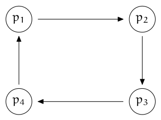
Answer
This Sage session gives equal values.
sage: H=matrix(QQ,[[0,0,0,1], [1,0,0,0], [0,1,0,0], [0,0,1,0]])
sage: S=matrix(QQ,[[1/4,1/4,1/4,1/4], [1/4,1/4,1/4,1/4], [1/4,1/4,1/4,1/4], [1/4,1/4,1/4,1/4]])
sage: alpha=0.85
sage: G=alpha*H+(1-alpha)*S
sage: I=matrix(QQ,[[1,0,0,0], [0,1,0,0], [0,0,1,0], [0,0,0,1]])
sage: N=G-I
sage: 1200*N
[-1155.00000000000  45.0000000000000  45.0000000000000  1065.00000000000]
[ 1065.00000000000 -1155.00000000000  45.0000000000000  45.0000000000000]
[ 45.0000000000000  1065.00000000000 -1155.00000000000  45.0000000000000]
[ 45.0000000000000  45.0000000000000  1065.00000000000 -1155.00000000000]
sage: M=matrix(QQ,[[-1155,45,45,1065], [1065,-1155,45,45], [45,1065,-1155,45], [45,45,1065,-1155]])
sage: M.echelon_form()
[ 1  0  0 -1]
[ 0  1  0 -1]
[ 0  0  1 -1]
[ 0  0  0  0]
sage: v=vector([1,1,1,1])
sage: (v/v.norm()).n()
(0.500000000000000, 0.500000000000000, 0.500000000000000, 0.500000000000000)
3 Topic: Page Ranking source ↗
[Bryan & Leise] Give the importance ranking for this web of pages.
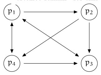
Use .
Use .
Observe that while is linked-to from all other pages, and therefore seems important, it is not the highest ranked page. What is the highest ranked page? Explain.
Answer (4 parts)
We have this.
This Sage session gives the answer.
sage: H=matrix(QQ,[[0,0,1,1/2], [1/3,0,0,0], [1/3,1/2,0,1/2], [1/3,1/2,0,0]])
sage: S=matrix(QQ,[[1/4,1/4,1/4,1/4], [1/4,1/4,1/4,1/4], [1/4,1/4,1/4,1/4], [1/4,1/4,1/4,1/4]])
sage: I=matrix(QQ,[[1,0,0,0], [0,1,0,0], [0,0,1,0], [0,0,0,1]])
sage: alpha=0.85
sage: G=alpha*H+(1-alpha)*S
sage: N=G-I
sage: 1200*N
[-1155.00000000000  45.0000000000000  1065.00000000000  555.000000000000]
[ 385.000000000000 -1155.00000000000  45.0000000000000  45.0000000000000]
[ 385.000000000000  555.000000000000 -1155.00000000000  555.000000000000]
[ 385.000000000000  555.000000000000  45.0000000000000 -1155.00000000000]
sage: M=matrix(QQ,[[-1155,45,1065,555], [385,-1155,45,45], [385,555,-1155,555],
....:      [385,555,45,-1155]])
sage: M.echelon_form()
[            1             0             0 -106613/58520]
[            0             1             0        -40/57]
[            0             0             1        -57/40]
[            0             0             0             0]
sage: v=vector([106613/58520,40/57,57/40,1])
sage: (v/v.norm()).n()
(0.696483066294572, 0.268280959381099, 0.544778023143244, 0.382300367118066)Continue the Sage session to get this.
 sage: alpha=0.95
sage: G=alpha*H+(1-alpha)*S
sage: N=G-I
sage: 1200*N
[-1185.00000000000  15.0000000000000  1155.00000000000  585.000000000000]
[ 395.000000000000 -1185.00000000000  15.0000000000000  15.0000000000000]
[ 395.000000000000  585.000000000000 -1185.00000000000  585.000000000000]
[ 395.000000000000  585.000000000000  15.0000000000000 -1185.00000000000]
sage: M=matrix(QQ,[[-1185,15,1155,585], [395,-1185,15,15], [395,585,-1185,585],
....:      [395,585,15,-1185]])
sage: M.echelon_form()
[             1              0              0 -361677/186440]
[             0              1              0         -40/59]
[             0              0              1         -59/40]
[             0              0              0              0]
sage: v=vector([361677/186440,40/59,59/40,1])
sage: (v/v.norm()).n()
(0.713196892748114, 0.249250262646952, 0.542275102671275, 0.367644137404254)Page is important, but it passes its importance on to only one page, . So that page receives a large boost.
1 Topic: Linear Recurrences source ↗
How many months until the number of Fibonacci rabbit pairs passes a thousand? Ten thousand? A million?
Answer
We use the formula
As observed earlier, is larger than one while has absolute value less than one.
sage: phi = (1+5^(0.5))/2
sage: psi = (1-5^(0.5))/2
sage: phi
1.61803398874989
sage: psi
-0.618033988749895
So the value of the expression is dominated by the first term. Solving gives this.
sage: a = ln(1000*5^(0.5))/ln(phi)
sage: a
16.0271918385296
sage: psi^(17)
-0.000280033582072583
So by the seventeenth power, the second term does not contribute enough to change the roundoff. For the ten thousand and million calculations the situation is even more extreme.
sage: b = ln(10000*5^(0.5))/ln(phi)
sage: b
20.8121638053112
sage: c = ln(1000000*5^(0.5))/ln(phi)
sage: c
30.3821077388746
The answers in these cases are and .
2 Topic: Linear Recurrences source ↗
Solve each homogeneous linear recurrence relations.
Answer (3 parts)
We express the relation in matrix form.
The characteristic equation of the matrix
has roots of and . Any function of the form satisfies the recurrence.
The matrix expression of the relation is
and the characteristic equation
has the two roots and . Any function of the form satisfies this recurrence.
In matrix form the relation
has a characteristic equation with roots , , and . Any combination of the form solves the recurrence.
3 Topic: Linear Recurrences source ↗
Give a formula for the relations of the prior exercise, with these initial conditions.
,
,
, , .
Answer (3 parts)
The solution of the homogeneous recurrence is . Substituting and gives this linear system.
By eye we see that and .
The solution of the homogeneous recurrence is . The initial conditions give this linear system.
The solution is , .
The homogeneous recurrence has the solution . With the initial conditions we get this linear system.
Its solution is , , .
4 Topic: Linear Recurrences source ↗
Check that the isomorphism given between and is a linear map.
Answer
Fix a linear homogeneous recurrence of order . Let be the set of functions satisfying the recurrence. Consider the function given as here.
This shows linearity.
5 Topic: Linear Recurrences source ↗
Show that the characteristic equation of the matrix is as stated, that is, is the polynomial associated with the relation. (Hint: expanding down the final column and using induction will work.)
Answer
We use the hint to prove this.
The base step is trivial. For the inductive step, expanding down the final column gives two nonzero terms.
(The matrix is square so the sign in front of is ). Application of the inductive hypothesis gives the desired result.
6 Topic: Linear Recurrences source ↗
Given a homogeneous linear recurrence relation , let , …, be the roots of the associated polynomial. Prove that each function satisfies the recurrence (without initial conditions).
Answer
This is a straightforward induction on .
7 Topic: Linear Recurrences source ↗
(This refers to the value given in the computer code below.) Transferring one disk per second, how many years would it take the priests at the Tower of Hanoi to finish the job?
Answer
Sage says that we are safe.
sage: T64 = 18446744073709551615
sage: T64_days = T64/(60*60*24)
sage: T64_days
1229782938247303441/5760
sage: T64_years = T64_days/365.25
sage: T64_years
5.84542046090626e11
sage: age_of_universe = 13.8e9
sage: T64_years/age_of_universe
42.3581192819294
1 Topic: Coupled Oscillators source ↗
Use the formula for the cosine of a sum to give an even more general formula for simple harmonic motion.
Answer
The angle sum formula for the cosine function is . Expand to . Then and do not vary with so we get the general solution .
2 Topic: Coupled Oscillators source ↗
Find the eigenvectors associated with the eigenvalues.
Answer
We will do the first root; the second is similar. We have this equation.
Plug in the first root . The two equations are redundant so we just consider the first.
That’s a line through the origin in the plane, so to specify it we need only find the ratio between the first and second variables.
So this is the space of eigenvectors associated with the first eigenvalue.
3 Topic: Coupled Oscillators source ↗
Find the values of in the case where and .
Answer
Observe that . Take the derivatives
and
and plug into the equations of motion ().
Factor out
and divide through by and .
We are assuming that and are equal, and writing for that number. Make the substitution and restate it as a matrix equation.
We want the frequencies for which this system has a nontrivial solution.
This is the same determinant as we did in the Topic body except that the second column is multiplied by . Multiplying a row or column by a scalar multiplies the entire determinant by that scalar. So this determinant is the negative of the one in the Topic body. But we are setting it to zero so that doesn’t matter. The roots are the same as in the Topic body.
4 Topic: Coupled Oscillators source ↗
Build a Wilberforce pendulum out of a Slinky Jr and a soup can. You can drill holes in the can for bolts, either two or four of them, that you can use to adjust the moment of inertia of the can so the periods of vertical and rotational motion coincide.
Answer
See [Mewes].
1 Topic: Inner Product source ↗
Verify that along with dot product is an inner product space.
Answer
The opening paragraph of this Topic notes that dot product is linear in both inputs, and so the first condition is satisfied. Condition (2) concerns conjugation, which has no effect on reals, and so this condition is trivially satisfied. Condition (3) requires that the length (the ordinary Euclidean length in -dimensional real space) be zero if and only if the vector is . If the vector has components , … then if and only if all the components are zero.
2 Topic: Inner Product source ↗
Show that Hermitian inner product on the two-dimensional vector space satisfies the three conditions in the definition of inner product.
Answer
The development in the Topic body proves (1) and (2). For (3), suppose that two members of have -th components and , so that . Then equals , which clearly equals if and only if each component is .
3 Topic: Inner Product source ↗
Show that this operation is an inner product on the real vector space .
Answer
Condition (1), linearity in the first argument, is easy.
Scalar multiplication is just as routine. Condition (2) concerns conjugation, which has no effect on reals and so this condition is trivially satisfied. For (3), of course , with equality if and only if each entry is zero.
4 Topic: Inner Product source ↗
Consider the real vector space of quadratic polynomials . Show that this is an inner product operation: . Consider the resulting norm. What is ?
Answer
Condition (1) is that it is linear in the first input. Verifying that this operation respects addition is routine
as is verifying that it respects scalar multiplication. Because this is a real vector space, and conjugation has no effect on real number scalars, it satisfies condition (2). For condition (3), let . Then is clearly non-negative, and is equal to if and only if is the zero polynomial.
As to the norm of , we have this.
5 Topic: Inner Product source ↗
Verify that the set of real valued functions that are continuous on the closed interval is a vector space.
Answer
The ten conditions in the definition of a vector space are consequences of results from Calculus. For example, the first condition is closure under addition and we have that the sum of two continuous functions is a continuous function in Calculus. (Although, often a student does not see a completely precise proof until a later class.) Similarly, addition of two functions is commutative. Of course, the zero vector is the function , which is continuous.
6 Topic: Inner Product source ↗
Show that an attempted definition of on that is linear in both inputs loses that gives the length.
Answer
Suppose that is greater than or equal to for all complex vectors . Then linearity in both inputs gives .
End of the book.
Exercises and answers are adapted from Linear Algebra by Jim Hefferon, which is free to read and download, and are used under the CC BY-SA 2.5 licence. They are taken from the book’s LaTeX source and set for the web, so they may differ slightly from the printed page. This adaptation is released under the same licence and is neither affiliated with nor endorsed by Jim Hefferon.