Every problem in the chapter beside the book’s answer, a chapter at a time as you scroll.
Chapter 1: Introduction to data
34 problems · 5 figuresGuided Practice 1.1 §1.1 source ↗
Of the 224 patients in the treatment group, 45 had a stroke by the end of the first year. Using these two numbers, compute the proportion of patients in the treatment group who had a stroke by the end of their first year. (Please note: answers to all Guided Practice exercises are provided using footnotes.)
Answer
The proportion of the 224 patients who had a stroke within 365 days: .
1.1 §1.1 source ↗
Migraine and acupuncture, Part I. A migraine is a particularly painful type of headache, which patients sometimes wish to treat with acupuncture. To determine whether acupuncture relieves migraine pain, researchers conducted a randomized controlled study where 89 females diagnosed with migraine headaches were randomly assigned to one of two groups: treatment or control. 43 patients in the treatment group received acupuncture that is specifically designed to treat migraines. 46 patients in the control group received placebo acupuncture (needle insertion at non-acupoint locations). 24 hours after patients received acupuncture, they were asked if they were pain free. Results are summarized in the contingency table below.
| Pain free | ||||
| Yes | No | Total | ||
| Treatment | 10 | 33 | 43 | |
| Group | Control | 2 | 44 | 46 |
| Total | 12 | 77 | 89 | |
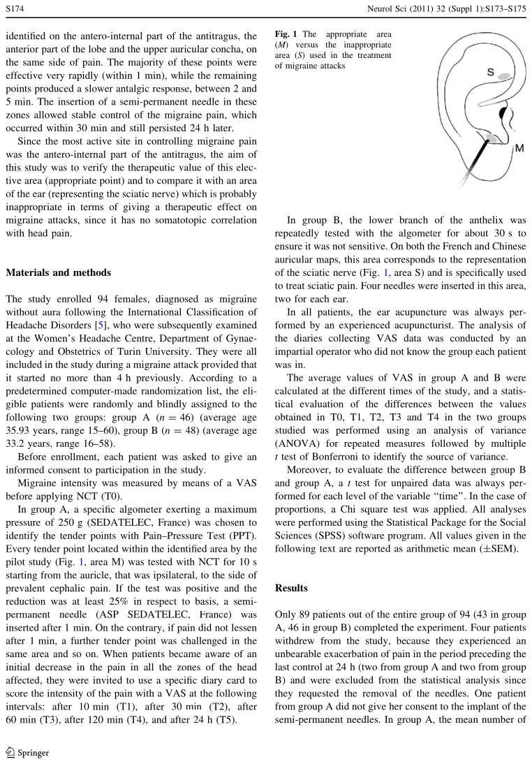
Figure from the original paper displaying the appropriate area (M) versus the inappropriate area (S) used in the treatment of migraine attacks.
What percent of patients in the treatment group were pain free 24 hours after receiving acupuncture?
What percent were pain free in the control group?
In which group did a higher percent of patients become pain free 24 hours after receiving acupuncture?
Your findings so far might suggest that acupuncture is an effective treatment for migraines for all people who suffer from migraines. However, this is not the only possible conclusion that can be drawn based on your findings so far. What is one other possible explanation for the observed difference between the percentages of patients that are pain free 24 hours after receiving acupuncture in the two groups?
Answer (4 parts)
Treatment: .
Control: .
A higher percentage of patients in the treatment group were pain free 24 hours after receiving acupuncture.
It is possible that the observed difference between the two group percentages is due to chance.
Guided Practice 1.2 §1.2 source ↗
What is the grade of the first loan in Figure 1.3? And what is the home ownership status of the borrower for that first loan? For these Guided Practice questions, you can check your answer in the footnote.
loan_amount | interest_rate | term | grade | state | total_income | homeownership | |
| 1 | 22000 | 10.90 | 60.00 | B | NJ | 59000.00 | rent |
| 2 | 6000 | 9.92 | 36.00 | B | CA | 60000.00 | rent |
| 3 | 25000 | 26.30 | 36.00 | E | SC | 75000.00 | mortgage |
| 50 | 15000 | 6.08 | 36.00 | A | TX | 77500.00 | mortgage |
loan50 data matrix.Answer
The loan’s grade is B, and the borrower rents their residence.
Guided Practice 1.3 §1.2 source ↗
The grades for assignments, quizzes, and exams in a course are often recorded in a gradebook that takes the form of a data matrix. How might you organize grade data using a data matrix?
Answer
There are multiple strategies that can be followed. One common strategy is to have each student represented by a row, and then add a column for each assignment, quiz, or exam. Under this setup, it is easy to review a single line to understand a student’s grade history. There should also be columns to include student information, such as one column to list student names.
Guided Practice 1.4 §1.2 source ↗
We consider data for 3,142 counties in the United States, which includes each county’s name, the state where it resides, its population in 2017, how its population changed from 2010 to 2017, poverty rate, and six additional characteristics. How might these data be organized in a data matrix?
Answer
Each county may be viewed as a case, and there are eleven pieces of information recorded for each case. A table with 3,142 rows and 11 columns could hold these data, where each row represents a county and each column represents a particular piece of information.
Guided Practice 1.6 §1.2 source ↗
An experiment is evaluating the effectiveness of a new drug in treating migraines. A group variable is used to indicate the experiment group for each patient: treatment or control. The num_migraines variable represents the number of migraines the patient experienced during a 3-month period. Classify each variable as either numerical or categorical.
Answer
The group variable can take just one of two group names, making it categorical. The num_migraines variable describes a count of the number of migraines, which is an outcome where basic arithmetic is sensible, which means this is numerical outcome; more specifically, since it represents a count, num_migraines is a discrete numerical variable.
Guided Practice 1.7 §1.2 source ↗
Examine the variables in the loan50 data set, which are described in Figure 1.4. Create two questions about possible relationships between variables in loan50 that are of interest to you.
| variable | description |
loan_amount | Amount of the loan received, in US dollars. |
interest_rate | Interest rate on the loan, in an annual percentage. |
term | The length of the loan, which is always set as a whole number of months. |
grade | Loan grade, which takes values A through G and represents the quality of the loan and its likelihood of being repaid. |
state | US state where the borrower resides. |
total_income | Borrower’s total income, including any second income, in US dollars. |
homeownership | Indicates whether the person owns, owns but has a mortgage, or rents. |
loan50 data set.Answer
Two example questions: (1) What is the relationship between loan amount and total income? (2) If someone’s income is above the average, will their interest rate tend to be above or below the average?
1.3 §1.2 source ↗
Air pollution and birth outcomes, study components. Researchers collected data to examine the relationship between air pollutants and preterm births in Southern California. During the study air pollution levels were measured by air quality monitoring stations. Specifically, levels of carbon monoxide were recorded in parts per million, nitrogen dioxide and ozone in parts per hundred million, and coarse particulate matter (PM) in . Length of gestation data were collected on 143,196 births between the years 1989 and 1993, and air pollution exposure during gestation was calculated for each birth. The analysis suggested that increased ambient PM and, to a lesser degree, CO concentrations may be associated with the occurrence of preterm births.
Identify the main research question of the study.
Who are the subjects in this study, and how many are included?
What are the variables in the study? Identify each variable as numerical or categorical. If numerical, state whether the variable is discrete or continuous. If categorical, state whether the variable is ordinal.
Answer (3 parts)
“Is there an association between air pollution exposure and preterm births?"
143,196 births in Southern California between 1989 and 1993.
Measurements of carbon monoxide, nitrogen dioxide, ozone, and particulate matter less than 10 (PM) collected at air-quality-monitoring stations as well as length of gestation. Continuous numerical variables.
1.5 §1.2 source ↗
Cheaters, study components. Researchers studying the relationship between honesty, age and self-control conducted an experiment on 160 children between the ages of 5 and 15. Participants reported their age, sex, and whether they were an only child or not. The researchers asked each child to toss a fair coin in private and to record the outcome (white or black) on a paper sheet, and said they would only reward children who report white. The study’s findings can be summarized as follows: “Half the students were explicitly told not to cheat and the others were not given any explicit instructions. In the no instruction group probability of cheating was found to be uniform across groups based on child’s characteristics. In the group that was explicitly told to not cheat, girls were less likely to cheat, and while rate of cheating didn’t vary by age for boys, it decreased with age for girls.”
Identify the main research question of the study.
Who are the subjects in this study, and how many are included?
How many variables were recorded for each subject in the study in order to conclude these findings? State the variables and their types.
Answer (3 parts)
“Does explicitly telling children not to cheat affect their likelihood to cheat?".
160 children between the ages of 5 and 15.
Four variables: (1) age (numerical, continuous), (2) sex (categorical), (3) whether they were an only child or not (categorical), (4) whether they cheated or not (categorical).
1.7 §1.2 source ↗
Migraine and acupuncture, Part II. Exercise 1.1 introduced a study exploring whether acupuncture had any effect on migraines. Researchers conducted a randomized controlled study where patients were randomly assigned to one of two groups: treatment or control. The patients in the treatment group received acupuncture that was specifically designed to treat migraines. The patients in the control group received placebo acupuncture (needle insertion at non-acupoint locations). 24 hours after patients received acupuncture, they were asked if they were pain free. What are the explanatory and response variables in this study?
Migraine and acupuncture, Part I. A migraine is a particularly painful type of headache, which patients sometimes wish to treat with acupuncture. To determine whether acupuncture relieves migraine pain, researchers conducted a randomized controlled study where 89 females diagnosed with migraine headaches were randomly assigned to one of two groups: treatment or control. 43 patients in the treatment group received acupuncture that is specifically designed to treat migraines. 46 patients in the control group received placebo acupuncture (needle insertion at non-acupoint locations). 24 hours after patients received acupuncture, they were asked if they were pain free. Results are summarized in the contingency table below.
| Pain free | ||||
| Yes | No | Total | ||
| Treatment | 10 | 33 | 43 | |
| Group | Control | 2 | 44 | 46 |
| Total | 12 | 77 | 89 | |
Figure from the original paper displaying the appropriate area (M) versus the inappropriate area (S) used in the treatment of migraine attacks.
(a) What percent of patients in the treatment group were pain free 24 hours after receiving acupuncture?
(b) What percent were pain free in the control group?
(c) In which group did a higher percent of patients become pain free 24 hours after receiving acupuncture?
(d) Your findings so far might suggest that acupuncture is an effective treatment for migraines for all people who suffer from migraines. However, this is not the only possible conclusion that can be drawn based on your findings so far. What is one other possible explanation for the observed difference between the percentages of patients that are pain free 24 hours after receiving acupuncture in the two groups?
Answer. (a) Treatment: .
(b) Control: . (c) A higher percentage of patients in the treatment group were pain free 24 hours after receiving acupuncture. (d) It is possible that the observed difference between the two group percentages is due to chance.
Answer
Explanatory: acupuncture or not. Response: if the patient was pain free or not.
1.9 §1.2 source ↗
Fisher’s irises. Sir Ronald Aylmer Fisher was an English statistician, evolutionary biologist, and geneticist who worked on a data set that contained sepal length and width, and petal length and width from three species of iris flowers (setosa, versicolor and virginica). There were 50 flowers from each species in the data set.
(a) How many cases were included in the data?
(b) How many numerical variables are included in the data? Indicate what they are, and if they are continuous or discrete.
(c) How many categorical variables are included in the data, and what are they? List the corresponding levels (categories).
Photo by Ryan Claussen (http://flic.kr/p/6QTcuX) CC BY-SA 2.0 license
Answer (3 parts)
.
Four continuous numerical variables: sepal length, sepal width, petal length, and petal width.
One categorical variable, species, with three levels: setosa, versicolor, and virginica.
1.11 §1.2 source ↗
US Airports. The visualization below shows the geographical distribution of airports in the contiguous United States and Washington, DC. This visualization was constructed based on a dataset where each observation is an airport.
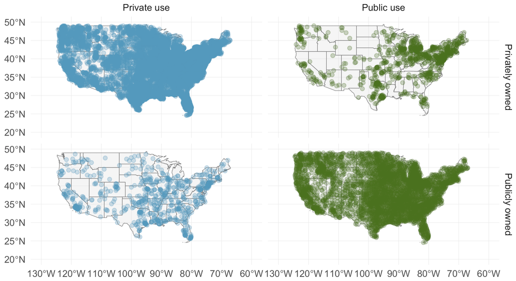
List the variables used in creating this visualization.
Indicate whether each variable in the study is numerical or categorical. If numerical, identify as continuous or discrete. If categorical, indicate if the variable is ordinal.
Answer (2 parts)
Airport ownership status (public/private), airport usage status (public/private), latitude, and longitude.
Airport ownership status: categorical, not ordinal. Airport usage status: categorical, not ordinal. Latitude: numerical, continuous. Longitude: numerical, continuous.
Guided Practice 1.9 §1.3 source ↗
For the second and third questions above, identify the target population and what represents an individual case.
Answer
(1.3.1) The first question is only relevant to students who complete their degree; the average cannot be computed using a student who never finished her degree. Thus, only Duke undergrads who graduated in the last five years represent cases in the population under consideration. Each such student is an individual case. (1.3.1) A person with severe heart disease represents a case. The population includes all people with severe heart disease.
Guided Practice 1.11 §1.3 source ↗
We can easily access ratings for products, sellers, and companies through websites. These ratings are based only on those people who go out of their way to provide a rating. If 50% of online reviews for a product are negative, do you think this means that 50% of buyers are dissatisfied with the product?
Answer
Answers will vary. From our own anecdotal experiences, we believe people tend to rant more about products that fell below expectations than rave about those that perform as expected. For this reason, we suspect there is a negative bias in product ratings on sites like Amazon. However, since our experiences may not be representative, we also keep an open mind.
Guided Practice 1.12 §1.3 source ↗
Suppose an observational study tracked sunscreen use and skin cancer, and it was found that the more sunscreen someone used, the more likely the person was to have skin cancer. Does this mean sunscreen causes skin cancer?
Answer
No. See the paragraph following the exercise for an explanation.
Guided Practice 1.13 §1.3 source ↗
Figure 1.8 shows a negative association between the homeownership rate and the percentage of multi-unit structures in a county. However, it is unreasonable to conclude that there is a causal relationship between the two variables. Suggest a variable that might explain the negative relationship.
Answer
Answers will vary. Population density may be important. If a county is very dense, then this may require a larger fraction of residents to live in multi-unit structures. Additionally, the high density may contribute to increases in property value, making homeownership infeasible for many residents.
1.13 §1.3 source ↗
Air pollution and birth outcomes, scope of inference. Exercise 1.3 introduces a study where researchers collected data to examine the relationship between air pollutants and preterm births in Southern California. During the study air pollution levels were measured by air quality monitoring stations. Length of gestation data were collected on 143,196 births between the years 1989 and 1993, and air pollution exposure during gestation was calculated for each birth.
Identify the population of interest and the sample in this study.
Comment on whether or not the results of the study can be generalized to the population, and if the findings of the study can be used to establish causal relationships.
Air pollution and birth outcomes, study components. Researchers collected data to examine the relationship between air pollutants and preterm births in Southern California. During the study air pollution levels were measured by air quality monitoring stations. Specifically, levels of carbon monoxide were recorded in parts per million, nitrogen dioxide and ozone in parts per hundred million, and coarse particulate matter (PM) in . Length of gestation data were collected on 143,196 births between the years 1989 and 1993, and air pollution exposure during gestation was calculated for each birth. The analysis suggested that increased ambient PM and, to a lesser degree, CO concentrations may be associated with the occurrence of preterm births.
(a) Identify the main research question of the study.
(b) Who are the subjects in this study, and how many are included?
(c) What are the variables in the study? Identify each variable as numerical or categorical. If numerical, state whether the variable is discrete or continuous. If categorical, state whether the variable is ordinal.
Answer. (a) “Is there an association between air pollution exposure and preterm births?" (b) 143,196 births in Southern California between 1989 and 1993. (c) Measurements of carbon monoxide, nitrogen dioxide, ozone, and particulate matter less than 10 (PM) collected at air-quality-monitoring stations as well as length of gestation. Continuous numerical variables.
Answer (2 parts)
Population: all births, sample: 143,196 births between 1989 and 1993 in Southern California.
If births in this time span at the geography can be considered to be representative of all births, then the results are generalizable to the population of Southern California. However, since the study is observational the findings cannot be used to establish causal relationships.
1.15 §1.3 source ↗
Buteyko method, scope of inference. Exercise 1.4 introduces a study on using the Buteyko shallow breathing technique to reduce asthma symptoms and improve quality of life. As part of this study 600 asthma patients aged 18-69 who relied on medication for asthma treatment were recruited and randomly assigned to two groups: one practiced the Buteyko method and the other did not. Those in the Buteyko group experienced, on average, a significant reduction in asthma symptoms and an improvement in quality of life.
Identify the population of interest and the sample in this study.
Comment on whether or not the results of the study can be generalized to the population, and if the findings of the study can be used to establish causal relationships.
Buteyko method, study components. The Buteyko method is a shallow breathing technique developed by Konstantin Buteyko, a Russian doctor, in 1952. Anecdotal evidence suggests that the Buteyko method can reduce asthma symptoms and improve quality of life. In a scientific study to determine the effectiveness of this method, researchers recruited 600 asthma patients aged 18-69 who relied on medication for asthma treatment. These patients were randomly split into two research groups: one practiced the Buteyko method and the other did not. Patients were scored on quality of life, activity, asthma symptoms, and medication reduction on a scale from 0 to 10. On average, the participants in the Buteyko group experienced a significant reduction in asthma symptoms and an improvement in quality of life.
(a) Identify the main research question of the study.
(b) Who are the subjects in this study, and how many are included?
(c) What are the variables in the study? Identify each variable as numerical or categorical. If numerical, state whether the variable is discrete or continuous. If categorical, state whether the variable is ordinal.
Answer (2 parts)
Population: all asthma patients aged 18-69 who rely on medication for asthma treatment. Sample: 600 such patients.
If the patients in this sample, who are likely not randomly sampled, can be considered to be representative of all asthma patients aged 18-69 who rely on medication for asthma treatment, then the results are generalizable to the population defined above. Additionally, since the study is experimental, the findings can be used to establish causal relationships.
1.17 §1.3 source ↗
Relaxing after work. The General Social Survey asked the question, “After an average work day, about how many hours do you have to relax or pursue activities that you enjoy?" to a random sample of 1,155 Americans. The average relaxing time was found to be 1.65 hours. Determine which of the following is an observation, a variable, a sample statistic (value calculated based on the observed sample), or a population parameter.
An American in the sample.
Number of hours spent relaxing after an average work day.
1.65.
Average number of hours all Americans spend relaxing after an average work day.
Answer (4 parts)
Observation.
Variable.
Sample statistic (mean).
Population parameter (mean).
1.19 §1.3 source ↗
Course satisfaction across sections. A large college class has 160 students. All 160 students attend the lectures together, but the students are divided into 4 groups, each of 40 students, for lab sections administered by different teaching assistants. The professor wants to conduct a survey about how satisfied the students are with the course, and he believes that the lab section a student is in might affect the student’s overall satisfaction with the course.
What type of study is this?
Suggest a sampling strategy for carrying out this study.
Answer (2 parts)
Observational.
Use stratified sampling to randomly sample a fixed number of students, say 10, from each section for a total sample size of 40 students.
1.21 §1.3 source ↗
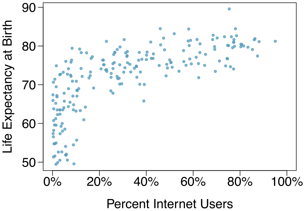
Internet use and life expectancy. The following scatterplot was created as part of a study evaluating the relationship between estimated life expectancy at birth (as of 2014) and percentage of internet users (as of 2009) in 208 countries for which such data were available.
(a) Describe the relationship between life expectancy and percentage of internet users.
(b) What type of study is this?
(c) State a possible confounding variable that might explain this relationship and describe its potential effect.
Answer (3 parts)
Positive, non-linear, somewhat strong. Countries in which a higher percentage of the population have access to the internet also tend to have higher average life expectancies, however rise in life expectancy trails off before around 80 years old.
Observational.
Wealth: countries with individuals who can widely afford the internet can probably also afford basic medical care. (Note: Answers may vary.)
1.23 §1.3 source ↗
Evaluate sampling methods. A university wants to determine what fraction of its undergraduate student body support a new $25 annual fee to improve the student union. For each proposed method below, indicate whether the method is reasonable or not.
Survey a simple random sample of 500 students.
Stratify students by their field of study, then sample 10% of students from each stratum.
Cluster students by their ages (e.g. 18 years old in one cluster, 19 years old in one cluster, etc.), then randomly sample three clusters and survey all students in those clusters.
Answer (3 parts)
Simple random sampling is okay. In fact, it’s rare for simple random sampling to not be a reasonable sampling method!
The student opinions may vary by field of study, so the stratifying by this variable makes sense and would be reasonable.
Students of similar ages are probably going to have more similar opinions, and we want clusters to be diverse with respect to the outcome of interest, so this would not be a good approach. (Additional thought: the clusters in this case may also have very different numbers of people, which can also create unexpected sample sizes.)
1.25 §1.3 source ↗
Haters are gonna hate, study confirms. A study published in the Journal of Personality and Social Psychology asked a group of 200 randomly sampled men and women to evaluate how they felt about various subjects, such as camping, health care, architecture, taxidermy, crossword puzzles, and Japan in order to measure their attitude towards mostly independent stimuli. Then, they presented the participants with information about a new product: a microwave oven. This microwave oven does not exist, but the participants didn’t know this, and were given three positive and three negative fake reviews. People who reacted positively to the subjects on the dispositional attitude measurement also tended to react positively to the microwave oven, and those who reacted negatively tended to react negatively to it. Researchers concluded that “some people tend to like things, whereas others tend to dislike things, and a more thorough understanding of this tendency will lead to a more thorough understanding of the psychology of attitudes."
What are the cases?
What is (are) the response variable(s) in this study?
What is (are) the explanatory variable(s) in this study?
Does the study employ random sampling?
Is this an observational study or an experiment? Explain your reasoning.
Can we establish a causal link between the explanatory and response variables?
Can the results of the study be generalized to the population at large?
Answer (7 parts)
The cases are 200 randomly sampled men and women.
The response variable is attitude towards a fictional microwave oven.
The explanatory variable is dispositional attitude.
Yes, the cases are sampled randomly.
This is an observational study since there is no random assignment to treatments.
No, we cannot establish a causal link between the explanatory and response variables since the study is observational.
Yes, the results of the study can be generalized to the population at large since the sample is random.
1.27 §1.3 source ↗
Sampling strategies. A statistics student who is curious about the relationship between the amount of time students spend on social networking sites and their performance at school decides to conduct a survey. Various research strategies for collecting data are described below. In each, name the sampling method proposed and any bias you might expect.
He randomly samples 40 students from the study’s population, gives them the survey, asks them to fill it out and bring it back the next day.
He gives out the survey only to his friends, making sure each one of them fills out the survey.
He posts a link to an online survey on Facebook and asks his friends to fill out the survey.
He randomly samples 5 classes and asks a random sample of students from those classes to fill out the survey.
Answer (4 parts)
Simple random sample. Non-response bias, if only those people who have strong opinions about the survey responds his sample may not be representative of the population.
Convenience sample. His sample may not be representative of the population since it consists only of his friends. It is also possible that the study will have non-response bias if some choose to not bring back the survey.
Convenience sample. This will have a similar issues to handing out surveys to friends.
Multi-stage sampling. If the classes are similar to each other with respect to student composition this approach should not introduce bias, other than potential non-response bias.
Guided Practice 1.16 §1.4 source ↗
Look back to the study in Section 1.1 where researchers were testing whether stents were effective at reducing strokes in at-risk patients. Is this an experiment? Was the study blinded? Was it double-blinded?
Answer
The researchers assigned the patients into their treatment groups, so this study was an experiment. However, the patients could distinguish what treatment they received, so this study was not blind. The study could not be double-blind since it was not blind.
Guided Practice 1.17 §1.4 source ↗
For the study in Section 1.1, could the researchers have employed a placebo? If so, what would that placebo have looked like?
Answer
Ultimately, can we make patients think they got treated from a surgery? In fact, we can, and some experiments use what’s called a sham surgery. In a sham surgery, the patient does undergo surgery, but the patient does not receive the full treatment, though they will still get a placebo effect.
1.29 §1.4 source ↗
Light and exam performance. A study is designed to test the effect of light level on exam performance of students. The researcher believes that light levels might have different effects on males and females, so wants to make sure both are equally represented in each treatment. The treatments are fluorescent overhead lighting, yellow overhead lighting, no overhead lighting (only desk lamps).
What is the response variable?
What is the explanatory variable? What are its levels?
What is the blocking variable? What are its levels?
Answer (3 parts)
Exam performance.
Light level: fluorescent overhead lighting, yellow overhead lighting, no overhead lighting (only desk lamps).
Sex: man, woman.
1.31 §1.4 source ↗
Light, noise, and exam performance. A study is designed to test the effect of light level and noise level on exam performance of students. The researcher believes that light and noise levels might have different effects on males and females, so wants to make sure both are equally represented in each treatment. The light treatments considered are fluorescent overhead lighting, yellow overhead lighting, no overhead lighting (only desk lamps). The noise treatments considered are no noise, construction noise, and human chatter noise.
What type of study is this?
How many factors are considered in this study? Identify them, and describe their levels.
What is the role of the sex variable in this study?
Answer (3 parts)
Experiment.
Light level (overhead lighting, yellow overhead lighting, no overhead lighting) and noise level (no noise, construction noise, and human chatter noise).
Since the researchers want to ensure equal gender representation, sex will be a blocking variable.
1.33 §1.4 source ↗
Soda preference. You would like to conduct an experiment in class to see if your classmates prefer the taste of regular Coke or Diet Coke. Briefly outline a design for this study.
Answer
Need randomization and blinding. One possible outline: (1) Prepare two cups for each participant, one containing regular Coke and the other containing Diet Coke. Make sure the cups are identical and contain equal amounts of soda. Label the cups A (regular) and B (diet). (Be sure to randomize A and B for each trial!) (2) Give each participant the two cups, one cup at a time, in random order, and ask the participant to record a value that indicates how much she liked the beverage. Be sure that neither the participant nor the person handing out the cups knows the identity of the beverage to make this a double- blind experiment. (Answers may vary.)
1.35 §1.R source ↗
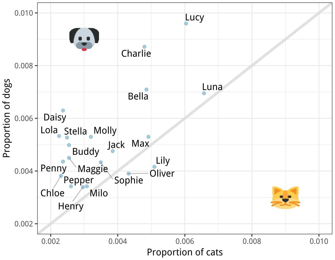
Pet names. The city of Seattle, WA has an open data portal that includes pets registered in the city. For each registered pet, we have information on the pet’s name and species. The following visualization plots the proportion of dogs with a given name versus the proportion of cats with the same name. The 20 most common cat and dog names are displayed. The diagonal line on the plot is the line; if a name appeared on this line, the name’s popularity would be exactly the same for dogs and cats.
(a) Are these data collected as part of an experiment or an observational study?
(b) What is the most common dog name? What is the most common cat name?
(c) What names are more common for cats than dogs?
(d) Is the relationship between the two variables positive or negative? What does this mean in context of the data?
Answer (4 parts)
Observational study.
Dog: Lucy. Cat: Luna.
Oliver and Lily.
Positive, as the popularity of a name for dogs increases, so does the popularity of that name for cats.
1.37 §1.R source ↗
Chia seeds and weight loss. Chia Pets – those terra-cotta figurines that sprout fuzzy green hair – made the chia plant a household name. But chia has gained an entirely new reputation as a diet supplement. In one 2009 study, a team of researchers recruited 38 men and divided them randomly into two groups: treatment or control. They also recruited 38 women, and they randomly placed half of these participants into the treatment group and the other half into the control group. One group was given 25 grams of chia seeds twice a day, and the other was given a placebo. The subjects volunteered to be a part of the study. After 12 weeks, the scientists found no significant difference between the groups in appetite or weight loss.
What type of study is this?
What are the experimental and control treatments in this study?
Has blocking been used in this study? If so, what is the blocking variable?
Has blinding been used in this study?
Comment on whether or not we can make a causal statement, and indicate whether or not we can generalize the conclusion to the population at large.
Answer (5 parts)
Experiment.
Treatment: 25 grams of chia seeds twice a day, control: placebo.
Yes, gender.
Yes, single blind since the patients were blinded to the treatment they received.
Since this is an experiment, we can make a causal statement. However, since the sample is not random, the causal statement cannot be generalized to the population at large.
1.39 §1.R source ↗
Flawed reasoning. Identify the flaw(s) in reasoning in the following scenarios. Explain what the individuals in the study should have done differently if they wanted to make such strong conclusions.
Students at an elementary school are given a questionnaire that they are asked to return after their parents have completed it. One of the questions asked is, “Do you find that your work schedule makes it difficult for you to spend time with your kids after school?" Of the parents who replied, 85% said “no". Based on these results, the school officials conclude that a great majority of the parents have no difficulty spending time with their kids after school.
A survey is conducted on a simple random sample of 1,000 women who recently gave birth, asking them about whether or not they smoked during pregnancy. A follow-up survey asking if the children have respiratory problems is conducted 3 years later. However, only 567 of these women are reached at the same address. The researcher reports that these 567 women are representative of all mothers.
An orthopedist administers a questionnaire to 30 of his patients who do not have any joint problems and finds that 20 of them regularly go running. He concludes that running decreases the risk of joint problems.
Answer (3 parts)
Non-responders may have a different response to this question, e.g. parents who returned the surveys likely don’t have difficulty spending time with their children.
It is unlikely that the women who were reached at the same address 3 years later are a random sample. These missing responders are probably renters (as opposed to homeowners) which means that they might be in a lower socio- economic status than the respondents.
There is no control group in this study, this is an observational study, and there may be confounding variables, e.g. these people may go running because they are generally healthier and/or do other exercises.
1.41 §1.R source ↗
Eat better, feel better? In a public health study on the effects of consumption of fruits and vegetables on psychological well-being in young adults, participants were randomly assigned to three groups: (1) diet-as-usual, (2) an ecological momentary intervention involving text message reminders to increase their fruits and vegetable consumption plus a voucher to purchase them, or (3) a fruit and vegetable intervention in which participants were given two additional daily servings of fresh fruits and vegetables to consume on top of their normal diet. Participants were asked to take a nightly survey on their smartphones. Participants were student volunteers at the University of Otago, New Zealand. At the end of the 14-day study, only participants in the third group showed improvements to their psychological well-being across the 14-days relative to the other groups.
What type of study is this?
Identify the explanatory and response variables.
Comment on whether the results of the study can be generalized to the population.
Comment on whether the results of the study can be used to establish causal relationships.
A newspaper article reporting on the study states, “The results of this study provide proof that giving young adults fresh fruits and vegetables to eat can have psychological benefits, even over a brief period of time.” How would you suggest revising this statement so that it can be supported by the study?
Answer (5 parts)
Randomized controlled experiment.
Explanatory: treatment group (categorical, with 3 levels). Response variable: Psychological well-being.
No, because the participants were volunteers.
Yes, because it was an experiment.
The statement should say “evidence” instead of “proof”.
1.43 §1.R source ↗
Stanford Open Policing. The Stanford Open Policing project gathers, analyzes, and releases records from traffic stops by law enforcement agencies across the United States. Their goal is to help researchers, journalists, and policymakers investigate and improve interactions between police and the public. The following is an excerpt from a summary table created based off of the data collected as part of this project.
| Driver’s | No. of stops | % of stopped | |||
| County | State | race | per year | cars searched | drivers arrested |
| Apaice County | Arizona | Black | 266 | 0.08 | 0.02 |
| Apaice County | Arizona | Hispanic | 1008 | 0.05 | 0.02 |
| Apaice County | Arizona | White | 6322 | 0.02 | 0.01 |
| Cochise County | Arizona | Black | 1169 | 0.05 | 0.01 |
| Cochise County | Arizona | Hispanic | 9453 | 0.04 | 0.01 |
| Cochise County | Arizona | White | 10826 | 0.02 | 0.01 |
| Wood County | Wisconsin | Black | 16 | 0.24 | 0.10 |
| Wood County | Wisconsin | Hispanic | 27 | 0.04 | 0.03 |
| Wood County | Wisconsin | White | 1157 | 0.03 | 0.03 |
What variables were collected on each individual traffic stop in order to create to the summary table above?
State whether each variable is numerical or categorical. If numerical, state whether it is continuous or discrete. If categorical, state whether it is ordinal or not.
Suppose we wanted to evaluate whether vehicle search rates are different for drivers of different races. In this analysis, which variable would be the response variable and which variable would be the explanatory variable?
Answer (3 parts)
Categorical, non-ordinal: County, State, Driver’s race. Numerical, discrete: No. of stops per year. Numerical, continuous: % searched, % drivers arrested.
All categorical, non-ordinal.
Response: whether the car was searched or not. Explanatory: race of the driver.
Loading chapter 2…
Exercises and answers are adapted from OpenIntro Statistics by David Diez, Mine Çetinkaya-Rundel and Christopher D Barr, which is free to read and download, and are used under the CC BY-SA 3.0 licence. They are taken from the book’s LaTeX source and set for the web, so they may differ slightly from the printed page. This adaptation is released under the same licence and is neither affiliated with nor endorsed by Diez, Çetinkaya-Rundel and Barr or OpenIntro.