Every problem in the chapter beside the book’s answer, a chapter at a time as you scroll.
Chapter 3: Probability
72 problems · 11 figuresGuided Practice 3.6 §3.1 source ↗
Random processes include rolling a die and flipping a coin.
Think of another random process.
Describe all the possible outcomes of that process. For instance, rolling a die is a random process with possible outcomes 1, 2, ..., 6.
Answer
Here are four examples. (i) Whether someone gets sick in the next month or not is an apparently random process with outcomes sick and not. (ii) We can generate a random process by randomly picking a person and measuring that person’s height. The outcome of this process will be a positive number. (iii) Whether the stock market goes up or down next week is a seemingly random process with possible outcomes up, down, and no_change. Alternatively, we could have used the percent change in the stock market as a numerical outcome. (iv) Whether your roommate cleans her dishes tonight probably seems like a random process with possible outcomes cleans_dishes and leaves_dishes.
Guided Practice 3.7 §3.1 source ↗
We are interested in the probability of rolling a 1, 4, or 5.
Explain why the outcomes 1, 4, and 5 are disjoint.
Apply the Addition Rule for disjoint outcomes to determine 1 or 4 or 5.
Answer (2 parts)
The random process is a die roll, and at most one of these outcomes can come up. This means they are disjoint outcomes.
1 or 4 or 5145
Guided Practice 3.8 §3.1 source ↗
In the loans data set in Chapter 2, the homeownership variable described whether the borrower rents, has a mortgage, or owns her property. Of the 10,000 borrowers, 3858 rented, 4789 had a mortgage, and 1353 owned their home.
1. Are the outcomes rent, mortgage, and own disjoint?
2. Determine the proportion of loans with value mortgage and own separately.
3. Use the Addition Rule for disjoint outcomes to compute the probability a randomly selected loan from the data set is for someone who has a mortgage or owns her home.
Answer (3 parts)
Yes. Each loan is categorized in only one level of homeownership.
Mortgage: . Own: .
mortgage or ownmortgageown.
Guided Practice 3.9 §3.1 source ↗
Verify the probability of event , , is using the Addition Rule.
Do the same for event .
Answer (2 parts)
1 or 212.
Similarly, .
Guided Practice 3.10 §3.1 source ↗
Using Figure 3.2 as a reference, what outcomes are represented by event ?
Are events and disjoint?
Are events and disjoint?
Answer (3 parts)
Outcomes 2 and 3.
Yes, events and are disjoint because they share no outcomes.
The events and share an outcome in common, 2, and so are not disjoint.
Guided Practice 3.11 §3.1 source ↗
In Guided Practice 3.10, you confirmed and from Figure 3.2 are disjoint. Compute the probability that event or event occurs.
(a) Using Figure 3.2 as a reference, what outcomes are represented by event ? (b) Are events and disjoint? (c) Are events and disjoint?
Answer. (a) Outcomes 2 and 3. (b) Yes, events and are disjoint because they share no outcomes. (c) The events and share an outcome in common, 2, and so are not disjoint.
Answer
Since and are disjoint events, use the Addition Rule: or .
Guided Practice 3.12 §3.1 source ↗
What is the probability that a randomly selected card is a diamond?
What is the probability that a randomly selected card is a face card?
Answer (2 parts)
There are 52 cards and 13 diamonds. If the cards are thoroughly shuffled, each card has an equal chance of being drawn, so the probability that a randomly selected card is a diamond is .
Likewise, there are 12 face cards, so face card.
Guided Practice 3.13 §3.1 source ↗
If and are disjoint, describe why this implies and .
Using part (a), verify that the General Addition Rule simplifies to the simpler Addition Rule for disjoint events if and are disjoint.
Answer (2 parts)
If and are disjoint, and can never occur simultaneously.
If and are disjoint, then the last term of in the General Addition Rule formula is 0 (see part (a)) and we are left with the Addition Rule for disjoint events.
Guided Practice 3.14 §3.1 source ↗
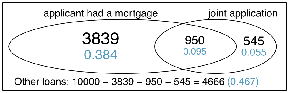
In the loans data set describing 10,000 loans, 1495 loans were from joint applications (e.g. a couple applied together), 4789 applicants had a mortgage, and 950 had both of these characteristics. Create a Venn diagram for this setup.
Answer
Both the counts and corresponding probabilities (e.g. ) are shown. Notice that the number of loans represented in the left circle corresponds to , and the number represented in the right circle is .
Guided Practice 3.15 §3.1 source ↗
Use your Venn diagram from Guided Practice 3.14 to determine the probability a randomly drawn loan from the loans data set is from a joint application where the couple had a mortgage.
What is the probability that the loan had either of these attributes?
In the loans data set describing 10,000 loans, 1495 loans were from joint applications (e.g. a couple applied together), 4789 applicants had a mortgage, and 950 had both of these characteristics. Create a Venn diagram for this setup.
Answer. Both the counts and corresponding probabilities (e.g. ) are shown. Notice that the number of loans represented in the left circle corresponds to , and the number represented in the right circle is .
Answer (2 parts)
The solution is represented by the intersection of the two circles: 0.095.
This is the sum of the three disjoint probabilities shown in the circles: (off by 0.001 due to a rounding error).
Guided Practice 3.16 §3.1 source ↗
Figure 3.6 suggests three distributions for household income in the United States. Only one is correct. Which one must it be? What is wrong with the other two?
| Income Range | $0-25k | $25k-50k | $50k-100k | $100k+ |
| (a) | 0.18 | 0.39 | 0.33 | 0.16 |
| (b) | 0.38 | -0.27 | 0.52 | 0.37 |
| (c) | 0.28 | 0.27 | 0.29 | 0.16 |
Answer (4 parts)
The probabilities of
do not sum to 1. The second probability in
is negative. This leaves
, which sure enough satisfies the requirements of a distribution. One of the three was said to be the actual distribution of US household incomes, so it must be (c).
Guided Practice 3.17 §3.1 source ↗
Compute rolling a 1, 4, 5, or 6.
What is ?
Answer (2 parts)
The outcomes are disjoint and each has probability , so the total probability is .
We can also see that . Since and are disjoint, .
Guided Practice 3.18 §3.1 source ↗
Events 1, 2 and 4, 6 are shown in Figure 3.2 on page .
Write out what and represent.
Compute and .
Compute and .
Answer (4 parts)
Brief solutions:
3, 4, 5, 6 and 1, 2, 3, 5.
Noting that each outcome is disjoint, add the individual outcome probabilities to get and .
and are disjoint, and the same is true of and . Therefore, and .
Guided Practice 3.19 §3.1 source ↗
Let represent the event where we roll two dice and their total is less than 12.
What does the event represent?
Determine from Figure 3.5 on page .
Determine .
| Dice sum | 2 | 3 | 4 | 5 | 6 | 7 | 8 | 9 | 10 | 11 | 12 |
| Probability |
Answer (3 parts)
The complement of : when the total is equal to 12.
.
Use the probability of the complement from part (b), , and the equation for the complement: less than 1212.
Guided Practice 3.20 §3.1 source ↗
Find the following probabilities for rolling two dice:
1. The sum of the dice is not 6.
2. The sum is at least 4. That is, determine the probability of the event 4, 5, ..., 12.
3. The sum is no more than 10. That is, determine the probability of the event 2, 3, ..., 10.
Answer (3 parts)
First find 6, then use the complement: not 66.
First find the complement, which requires much less effort: 2 or 3. Then calculate .
As before, finding the complement is the clever way to determine . First find 11 or 12. Then calculate .
Guided Practice 3.22 §3.1 source ↗
About 9% of people are left-handed. Suppose 2 people are selected at random from the U.S. population. Because the sample size of 2 is very small relative to the population, it is reasonable to assume these two people are independent.
What is the probability that both are left-handed?
What is the probability that both are right-handed?
Answer (2 parts)
The probability the first person is left-handed is , which is the same for the second person. We apply the Multiplication Rule for independent processes to determine the probability that both will be left-handed: .
It is reasonable to assume the proportion of people who are ambidextrous (both right- and left-handed) is nearly 0, which results in right-handed. Using the same reasoning as in part (a), the probability that both will be right-handed is .
Guided Practice 3.23 §3.1 source ↗
Suppose 5 people are selected at random.
(a) What is the probability that all are right-handed?
(b) What is the probability that all are left-handed?
(c) What is the probability that not all of the people are right-handed?
Answer (3 parts)
The abbreviations RH and LH are used for right-handed and left-handed, respectively. Since each are independent, we apply the Multiplication Rule for independent processes:
Using the same reasoning as in (a),
Use the complement, all five are RH, to answer this question:
Guided Practice 3.24 §3.1 source ↗
Three people are selected at random.
(a) What is the probability that the first person is male and right-handed?
(b) What is the probability that the first two people are male and right-handed?.
(c) What is the probability that the third person is female and left-handed?
(d) What is the probability that the first two people are male and right-handed and the third person is female and left-handed?
Answer (5 parts)
Brief answers are provided.
This can be written in probability notation as a randomly selected person is male and right-handed.
0.207.
0.045.
0.0093.
3.1 §3.1 source ↗
True or false. Determine if the statements below are true or false, and explain your reasoning.
If a fair coin is tossed many times and the last eight tosses are all heads, then the chance that the next toss will be heads is somewhat less than 50%.
Drawing a face card (jack, queen, or king) and drawing a red card from a full deck of playing cards are mutually exclusive events.
Drawing a face card and drawing an ace from a full deck of playing cards are mutually exclusive events.
Answer (3 parts)
False. These are independent trials.
False. There are red face cards.
True. A card cannot be both a face card and an ace.
3.3 §3.1 source ↗
Four games, one winner. Below are four versions of the same game. Your archnemesis gets to pick the version of the game, and then you get to choose how many times to flip a coin: 10 times or 100 times. Identify how many coin flips you should choose for each version of the game. It costs $1 to play each game. Explain your reasoning.
If the proportion of heads is larger than 0.60, you win $1.
If the proportion of heads is larger than 0.40, you win $1.
If the proportion of heads is between 0.40 and 0.60, you win $1.
If the proportion of heads is smaller than 0.30, you win $1.
Answer (4 parts)
10 tosses. Fewer tosses mean more variability in the sample fraction of heads, meaning there’s a better chance of getting at least 60% heads.
100 tosses. More flips means the observed proportion of heads would often be closer to the average, 0.50, and therefore also above 0.40.
100 tosses. With more flips, the observed proportion of heads would often be closer to the average, 0.50.
10 tosses. Fewer flips would increase variability in the fraction of tosses that are heads.
3.5 §3.1 source ↗
Coin flips. If you flip a fair coin 10 times, what is the probability of
getting all tails?
getting all heads?
getting at least one tails?
Answer (3 parts)
= 0.00098.
= 0.00098.
(at least one tails) = (no tails) = .
3.7 §3.1 source ↗
Swing voters. A Pew Research survey asked 2,373 randomly sampled registered voters their political affiliation (Republican, Democrat, or Independent) and whether or not they identify as swing voters. 35% of respondents identified as Independent, 23% identified as swing voters, and 11% identified as both.
Are being Independent and being a swing voter disjoint, i.e. mutually exclusive?
Draw a Venn diagram summarizing the variables and their associated probabilities.
What percent of voters are Independent but not swing voters?
What percent of voters are Independent or swing voters?
What percent of voters are neither Independent nor swing voters?
Is the event that someone is a swing voter independent of the event that someone is a political Independent?
Answer (6 parts)
No, there are voters who are both independent and swing voters.
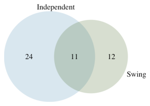
Each Independent voter is either a swing voter or not. Since 35% of voters are Independents and 11% are both Independent and swing voters, the other 24% must not be swing voters.
0.47.
0.53.
P(Independent) P(swing) = , which does not equal P(Independent and swing) = 0.11, so the events are dependent.
3.9 §3.1 source ↗
Disjoint vs. independent. In parts (a) and (b), identify whether the events are disjoint, independent, or neither (events cannot be both disjoint and independent).
You and a randomly selected student from your class both earn A’s in this course.
You and your class study partner both earn A’s in this course.
If two events can occur at the same time, must they be dependent?
Answer (3 parts)
If the class is not graded on a curve, they are independent. If graded on a curve, then neither independent nor disjoint – unless the instructor will only give one A, which is a situation we will ignore in parts
and
. (b) They are probably not independent: if you study together, your study habits would be related, which suggests your course performances are also related. (c) No. See the answer to part (a) when the course is not graded on a curve. More generally: if two things are unrelated (independent), then one occurring does not preclude the other from occurring.
3.11 §3.1 source ↗
Educational attainment of couples. The table below shows the distribution of education level attained by US residents by gender based on data collected in the 2010 American Community Survey.
| Gender | |||
| Male | Female | ||
| Less than 9th grade | 0.07 | 0.13 | |
| 9th to 12th grade, no diploma | 0.10 | 0.09 | |
| Highest | HS graduate (or equivalent) | 0.30 | 0.20 |
| education | Some college, no degree | 0.22 | 0.24 |
| attained | Associate’s degree | 0.06 | 0.08 |
| Bachelor’s degree | 0.16 | 0.17 | |
| Graduate or professional degree | 0.09 | 0.09 | |
| Total | 1.00 | 1.00 | |
What is the probability that a randomly chosen man has at least a Bachelor’s degree?
What is the probability that a randomly chosen woman has at least a Bachelor’s degree?
What is the probability that a man and a woman getting married both have at least a Bachelor’s degree? Note any assumptions you must make to answer this question.
If you made an assumption in part (c), do you think it was reasonable? If you didn’t make an assumption, double check your earlier answer and then return to this part.
Answer (4 parts)
.
.
Assuming that the education level of the husband and wife are independent: . You might also notice we actually made a second assumption: that the decision to get married is unrelated to education level.
The husband/wife independence assumption is probably not reasonable, because people often marry another person with a comparable level of education. We will leave it to you to think about whether the second assumption noted in part (c) is reasonable.
Guided Practice 3.28 §3.2 source ↗
Verify Figure 3.14 represents a probability distribution: events are disjoint, all probabilities are non-negative, and the probabilities sum to 1.
| Joint outcome | Probability |
mach_learn is pred_fashion
and truth is fashion | 0.1081 |
mach_learn is pred_fashion
and truth is not | 0.0121 |
mach_learn is pred_not
and truth is fashion | 0.0615 |
mach_learn is pred_not
and truth is not | 0.8183 |
| Total | 1.0000 |
photo_classify data set.Answer
Each of the four outcome combination are disjoint, all probabilities are indeed non-negative, and the sum of the probabilities is .
Guided Practice 3.29 §3.2 source ↗
Write out the following statement in conditional probability notation: “The probability that the ML prediction was correct, if the photo was about fashion”. Here the condition is now based on the photo’s truth status, not the ML algorithm.
Determine the probability from part (a). Table 3.13 may be helpful.
truth: fashion | truth: not | Total | |
mach_learn: pred_fashion | 0.1081 | 0.0121 | 0.1202 |
mach_learn: pred_not | 0.0615 | 0.8183 | 0.8798 |
| Total | 0.1696 | 0.8304 | 1.00 |
photo_classify data set.Answer (2 parts)
If the photo is about fashion and the ML algorithm prediction was correct, then the ML algorithm my have a value of pred_fashion:
The equation for conditional probability indicates we should first find
and .
Then the ratio represents the conditional probability: .
Guided Practice 3.30 §3.2 source ↗
Determine the probability that the algorithm is incorrect if it is known the photo is about fashion.
Using the answers from part (a) and Guided Practice 3.29(b), compute
Provide an intuitive argument to explain why the sum in (b) is 1.
(a) Write out the following statement in conditional probability notation: “The probability that the ML prediction was correct, if the photo was about fashion”. Here the condition is now based on the photo’s truth status, not the ML algorithm.
(b) Determine the probability from part (a). Table 3.13 may be helpful.
Answer. (a) If the photo is about fashion and the ML algorithm prediction was correct, then the ML algorithm my have a value of pred_fashion:
(b) The equation for conditional probability indicates we should first find
and .
Then the ratio represents the conditional probability: .
Answer (3 parts)
This probability is .
The total equals 1.
Under the condition the photo is about fashion, the ML algorithm must have either predicted it was about fashion or predicted it was not about fashion. The complement still works for conditional probabilities, provided the probabilities are conditioned on the same information.
Guided Practice 3.31 §3.2 source ↗
Write out, in formal notation, the probability a randomly selected person who was not inoculated died from smallpox, and find this probability.
Answer
result = died inoculated = no .
Guided Practice 3.32 §3.2 source ↗
Determine the probability that an inoculated person died from smallpox. How does this result compare with the result of Guided Practice 3.31?
Write out, in formal notation, the probability a randomly selected person who was not inoculated died from smallpox, and find this probability.
Answer. result = died inoculated = no .
Answer
result = died inoculated = yes (if we avoided rounding errors, we’d get ). The death rate for individuals who were inoculated is only about 1 in 40 while the death rate is about 1 in 7 for those who were not inoculated.
Guided Practice 3.33 §3.2 source ↗
The people of Boston self-selected whether or not to be inoculated.
Is this study observational or was this an experiment?
Can we infer any causal connection using these data?
What are some potential confounding variables that might influence whether someone lived or died and also affect whether that person was inoculated?
Answer (4 parts)
Brief answers:
Observational.
No, we cannot infer causation from this observational study.
Accessibility to the latest and best medical care. There are other valid answers for part (c).
Guided Practice 3.35 §3.2 source ↗
Use inoculated = yes and result = lived inoculated = yes to determine the probability that a person was both inoculated and lived.
Answer
The answer is 0.0382, which can be verified using Figure 3.16.
| inoculated | ||||
| yes | no | Total | ||
| lived | 0.0382 | 0.8252 | 0.8634 | |
result | died | 0.0010 | 0.1356 | 0.1366 |
| Total | 0.0392 | 0.9608 | 1.0000 | |
smallpox data, computed by dividing each count by the table total, 6224.Guided Practice 3.36 §3.2 source ↗
If 97.54% of the inoculated people lived, what proportion of inoculated people must have died?
Answer
There were only two possible outcomes: lived or died. This means that 100% - 97.54% = 2.46% of the people who were inoculated died.
Guided Practice 3.37 §3.2 source ↗
Based on the probabilities computed above, does it appear that inoculation is effective at reducing the risk of death from smallpox?
Answer
The samples are large relative to the difference in death rates for the “inoculated” and “not inoculated” groups, so it seems there is an association between inoculated and outcome. However, as noted in the solution to Guided Practice 3.33, this is an observational study and we cannot be sure if there is a causal connection. (Further research has shown that inoculation is effective at reducing death rates.)
The people of Boston self-selected whether or not to be inoculated. (a) Is this study observational or was this an experiment? (b) Can we infer any causal connection using these data? (c) What are some potential confounding variables that might influence whether someone lived or died and also affect whether that person was inoculated?
Answer. Brief answers: (a) Observational. (b) No, we cannot infer causation from this observational study. (c) Accessibility to the latest and best medical care. There are other valid answers for part (c).
Guided Practice 3.38 §3.2 source ↗
Let and represent the outcomes of rolling two dice.
1. What is the probability that the first die, , is 1?
2. What is the probability that both and are 1?
3. Use the formula for conditional probability to compute 1 1.
4. What is ? Is this different from the answer from part (c)? Explain.
Answer (5 parts)
Brief solutions:
.
.
.
The probability is the same as in part (c): . The probability that was unchanged by knowledge about , which makes sense as and are independent.
Guided Practice 3.39 §3.2 source ↗
Ron is watching a roulette table in a casino and notices that the last five outcomes were black. He figures that the chances of getting black six times in a row is very small (about ) and puts his paycheck on red. What is wrong with his reasoning?
Answer
He has forgotten that the next roulette spin is independent of the previous spins. Casinos do employ this practice, posting the last several outcomes of many betting games to trick unsuspecting gamblers into believing the odds are in their favor. This is called the gambler’s fallacy.
Guided Practice 3.41 §3.2 source ↗
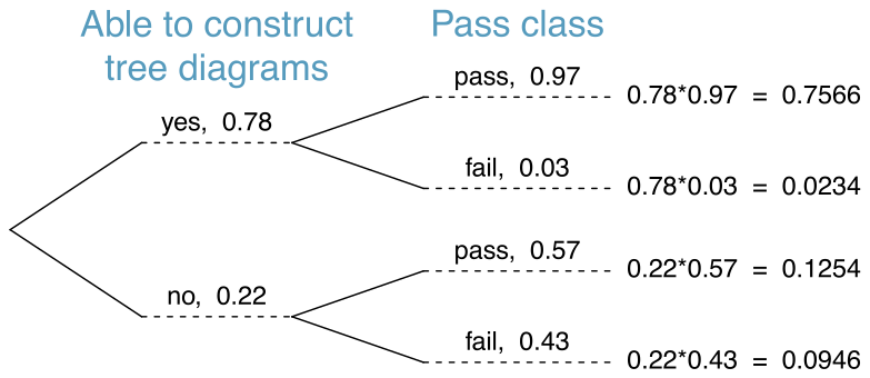
After an introductory statistics course, 78% of students can successfully construct tree diagrams. Of those who can construct tree diagrams, 97% passed, while only 57% of those students who could not construct tree diagrams passed.
Organize this information into a tree diagram.
What is the probability that a randomly selected student passed?
Compute the probability a student is able to construct a tree diagram if it is known that she passed.
Answer (3 parts)
The tree diagram is shown to the right.
Identify which two joint probabilities represent students who passed, and add them: passed.
construct tree diagram passed.
Guided Practice 3.43 §3.2 source ↗
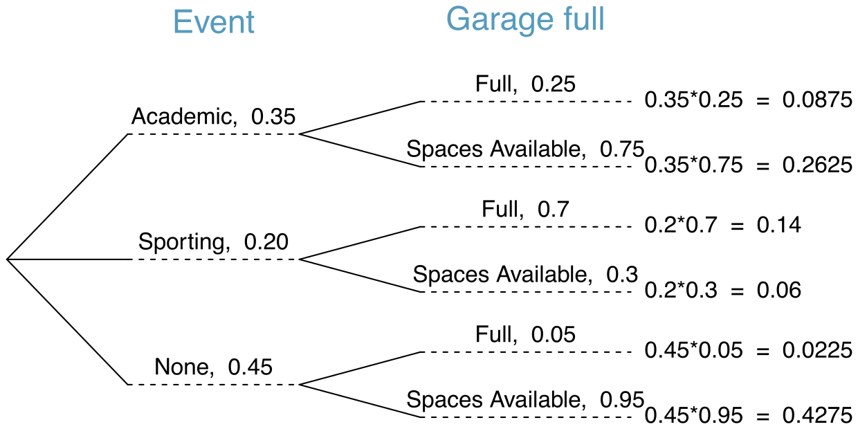
Jose visits campus every Thursday evening. However, some days the parking garage is full, often due to college events. There are academic events on 35% of evenings, sporting events on 20% of evenings, and no events on 45% of evenings. When there is an academic event, the garage fills up about 25% of the time, and it fills up 70% of evenings with sporting events. On evenings when there are no events, it only fills up about 5% of the time. If Jose comes to campus and finds the garage full, what is the probability that there is a sporting event? Use a tree diagram to solve this problem.
Answer
The tree diagram, with three primary branches, is shown to the right. Next, we identify two probabilities from the tree diagram. (1) The probability that there is a sporting event and the garage is full: 0.14. (2) The probability the garage is full: . Then the solution is the ratio of these probabilities: . If the garage is full, there is a 56% probability that there is a sporting event.
Guided Practice 3.45 §3.2 source ↗
Use the information in the previous exercise and example to verify the probability that there is an academic event conditioned on the parking lot being full is 0.35.
Answer
Short answer:
Guided Practice 3.46 §3.2 source ↗
In Guided Practice 3.43 and 3.45, you found that if the parking lot is full, the probability there is a sporting event is 0.56 and the probability there is an academic event is 0.35. Using this information, compute no event the lot is full.
Jose visits campus every Thursday evening. However, some days the parking garage is full, often due to college events. There are academic events on 35% of evenings, sporting events on 20% of evenings, and no events on 45% of evenings. When there is an academic event, the garage fills up about 25% of the time, and it fills up 70% of evenings with sporting events. On evenings when there are no events, it only fills up about 5% of the time. If Jose comes to campus and finds the garage full, what is the probability that there is a sporting event? Use a tree diagram to solve this problem.
Answer. The tree diagram, with three primary branches, is shown to the right. Next, we identify two probabilities from the tree diagram. (1) The probability that there is a sporting event and the garage is full: 0.14. (2) The probability the garage is full: . Then the solution is the ratio of these probabilities: . If the garage is full, there is a 56% probability that there is a sporting event.
Use the information in the previous exercise and example to verify the probability that there is an academic event conditioned on the parking lot being full is 0.35.
Answer. Short answer:
Answer
Each probability is conditioned on the same information that the garage is full, so the complement may be used: .
3.13 §3.2 source ↗
Joint and conditional probabilities. P(A) = 0.3, P(B) = 0.7
Can you compute P(A and B) if you only know P(A) and P(B)?
Assuming that events A and B arise from independent random processes,
(i) what is P(A and B)?
(ii) what is P(A or B)?
(iii) what is P(AB)?
If we are given that P(A and B) = 0.1, are the random variables giving rise to events A and B independent?
If we are given that P(A and B) = 0.1, what is P(AB)?
Answer
(a) No, but we could if A and B are independent. (b-i) 0.21. (b-ii) 0.79. (b-iii) 0.3. (c) No, because 0.1 0.21, where 0.21 was the value computed under independence from part (a). (d) 0.143.
3.15 §3.2 source ↗
Global warming. A Pew Research poll asked 1,306 Americans “From what you’ve read and heard, is there solid evidence that the average temperature on earth has been getting warmer over the past few decades, or not?". The table below shows the distribution of responses by party and ideology, where the counts have been replaced with relative frequencies.
| Response | |||||
| Earth is | Not | Don’t Know | |||
| warming | warming | Refuse | Total | ||
| Conservative Republican | 0.11 | 0.20 | 0.02 | 0.33 | |
| Party and | Mod/Lib Republican | 0.06 | 0.06 | 0.01 | 0.13 |
| Ideology | Mod/Cons Democrat | 0.25 | 0.07 | 0.02 | 0.34 |
| Liberal Democrat | 0.18 | 0.01 | 0.01 | 0.20 | |
| Total | 0.60 | 0.34 | 0.06 | 1.00 | |
Are believing that the earth is warming and being a liberal Democrat mutually exclusive?
What is the probability that a randomly chosen respondent believes the earth is warming or is a liberal Democrat?
What is the probability that a randomly chosen respondent believes the earth is warming given that he is a liberal Democrat?
What is the probability that a randomly chosen respondent believes the earth is warming given that he is a conservative Republican?
Does it appear that whether or not a respondent believes the earth is warming is independent of their party and ideology? Explain your reasoning.
What is the probability that a randomly chosen respondent is a moderate/liberal Republican given that he does not believe that the earth is warming?
Answer (6 parts)
No, 0.18 of respondents fall into this combination.
.
.
.
No, otherwise the answers to (c) and (d) would be the same.
.
3.17 §3.2 source ↗
Burger preferences. A 2010 SurveyUSA poll asked 500 Los Angeles residents, “What is the best hamburger place in Southern California? Five Guys Burgers? In-N-Out Burger? Fat Burger? Tommy’s Hamburgers? Umami Burger? Or somewhere else?” The distribution of responses by gender is shown below.
| Gender | ||||
| Male | Female | Total | ||
| Five Guys Burgers | 5 | 6 | 11 | |
| In-N-Out Burger | 162 | 181 | 343 | |
| Best | Fat Burger | 10 | 12 | 22 |
| hamburger | Tommy’s Hamburgers | 27 | 27 | 54 |
| place | Umami Burger | 5 | 1 | 6 |
| Other | 26 | 20 | 46 | |
| Not Sure | 13 | 5 | 18 | |
| Total | 248 | 252 | 500 | |
Are being female and liking Five Guys Burgers mutually exclusive?
What is the probability that a randomly chosen male likes In-N-Out the best?
What is the probability that a randomly chosen female likes In-N-Out the best?
What is the probability that a man and a woman who are dating both like In-N-Out the best? Note any assumption you make and evaluate whether you think that assumption is reasonable.
What is the probability that a randomly chosen person likes Umami best or that person is female?
Answer (5 parts)
No. There are 6 females who like Five Guys Burgers.
.
.
Under the assumption of a dating choices being independent of hamburger preference, which on the surface seems reasonable: .
.
3.19 §3.2 source ↗
Drawing box plots. After an introductory statistics course, 80% of students can successfully construct box plots. Of those who can construct box plots, 86% passed, while only 65% of those students who could not construct box plots passed.
Construct a tree diagram of this scenario.
Calculate the probability that a student is able to construct a box plot if it is known that he passed.
Answer (2 parts)
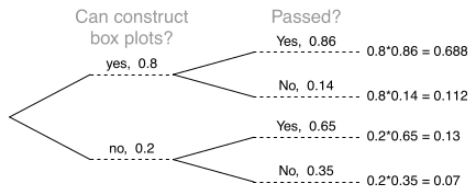
0.84
3.21 §3.2 source ↗
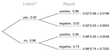
It’s never lupus. Lupus is a medical phenomenon where antibodies that are supposed to attack foreign cells to prevent infections instead see plasma proteins as foreign bodies, leading to a high risk of blood clotting. It is believed that 2% of the population suffer from this disease. The test is 98% accurate if a person actually has the disease. The test is 74% accurate if a person does not have the disease. There is a line from the Fox television show House that is often used after a patient tests positive for lupus: “It’s never lupus." Do you think there is truth to this statement? Use appropriate probabilities to support your answer.
Answer
0.0714. Even when a patient tests positive for lupus, there is only a 7.14% chance that he actually has lupus. House may be right.
Guided Practice 3.49 §3.3 source ↗
What rule permitted us to multiply the probabilities in Example 3.48?
If the professor asks 3 questions, what is the probability that you will not be selected? Assume that she will not pick the same person twice in a given lecture.
Answer. For the first question, she will pick someone else with probability . When she asks the second question, she only has 14 people who have not yet been asked. Thus, if you were not picked on the first question, the probability you are again not picked is . Similarly, the probability you are again not picked on the third question is , and the probability of not being picked for any of the three questions is
Answer
The three probabilities we computed were actually one marginal probability, Q1not_picked, and two conditional probabilities:
Using the General Multiplication Rule, the product of these three probabilities is the probability of not being picked in 3 questions.
Guided Practice 3.51 §3.3 source ↗
Under the setup of Example 3.50, what is the probability of being picked to answer all three questions?
Suppose the professor randomly picks without regard to who she already selected, i.e. students can be picked more than once. What is the probability that you will not be picked for any of the three questions?
Answer. Each pick is independent, and the probability of not being picked for any individual question is . Thus, we can use the Multiplication Rule for independent processes.
You have a slightly higher chance of not being picked compared to when she picked a new person for each question. However, you now may be picked more than once.
Answer
being picked to answer all three questions.
Guided Practice 3.52 §3.3 source ↗
Your department is holding a raffle. They sell 30 tickets and offer seven prizes.
They place the tickets in a hat and draw one for each prize. The tickets are sampled without replacement, i.e. the selected tickets are not placed back in the hat. What is the probability of winning a prize if you buy one ticket?
What if the tickets are sampled with replacement?
Answer (2 parts)
First determine the probability of not winning. The tickets are sampled without replacement, which means the probability you do not win on the first draw is , for the second, ..., and for the seventh. The probability you win no prize is the product of these separate probabilities: . That is, the probability of winning a prize is .
When the tickets are sampled with replacement, there are seven independent draws. Again we first find the probability of not winning a prize: . Thus, the probability of winning (at least) one prize when drawing with replacement is 0.211.
Guided Practice 3.53 §3.3 source ↗
Compare your answers in Guided Practice 3.52. How much influence does the sampling method have on your chances of winning a prize?
Your department is holding a raffle. They sell 30 tickets and offer seven prizes. (a) They place the tickets in a hat and draw one for each prize. The tickets are sampled without replacement, i.e. the selected tickets are not placed back in the hat. What is the probability of winning a prize if you buy one ticket? (b) What if the tickets are sampled with replacement?
Answer. (a) First determine the probability of not winning. The tickets are sampled without replacement, which means the probability you do not win on the first draw is , for the second, ..., and for the seventh. The probability you win no prize is the product of these separate probabilities: . That is, the probability of winning a prize is . (b) When the tickets are sampled with replacement, there are seven independent draws. Again we first find the probability of not winning a prize: . Thus, the probability of winning (at least) one prize when drawing with replacement is 0.211.
Answer
There is about a 10% larger chance of winning a prize when using sampling without replacement. However, at most one prize may be won under this sampling procedure.
3.23 §3.3 source ↗
Marbles in an urn. Imagine you have an urn containing 5 red, 3 blue, and 2 orange marbles in it.
What is the probability that the first marble you draw is blue?
Suppose you drew a blue marble in the first draw. If drawing with replacement, what is the probability of drawing a blue marble in the second draw?
Suppose you instead drew an orange marble in the first draw. If drawing with replacement, what is the probability of drawing a blue marble in the second draw?
If drawing with replacement, what is the probability of drawing two blue marbles in a row?
When drawing with replacement, are the draws independent? Explain.
Answer (5 parts)
0.3.
0.3.
0.3.
.
Yes, the population that is being sampled from is identical in each draw.
3.25 §3.3 source ↗
Chips in a bag. Imagine you have a bag containing 5 red, 3 blue, and 2 orange chips.
Suppose you draw a chip and it is blue. If drawing without replacement, what is the probability the next is also blue?
Suppose you draw a chip and it is orange, and then you draw a second chip without replacement. What is the probability this second chip is blue?
If drawing without replacement, what is the probability of drawing two blue chips in a row?
When drawing without replacement, are the draws independent? Explain.
Answer (4 parts)
.
.
.
No, e.g. in this exercise, removing one chip meaningfully changes the probability of what might be drawn next.
3.27 §3.3 source ↗
Student outfits. In a classroom with 24 students, 7 students are wearing jeans, 4 are wearing shorts, 8 are wearing skirts, and the rest are wearing leggings. If we randomly select 3 students without replacement, what is the probability that one of the selected students is wearing leggings and the other two are wearing jeans? Note that these are mutually exclusive clothing options.
Answer
leggings, jeans, jeans. However, the person with leggings could have come 2nd or 3rd, and these each have this same probability, so .
Guided Practice 3.55 §3.4 source ↗
Would you be surprised if the bookstore sold slightly more or less than 105 books?
Answer
If they sell a little more or a little less, this should not be a surprise. Hopefully Chapter 1 helped make clear that there is natural variability in observed data. For example, if we would flip a coin 100 times, it will not usually come up heads exactly half the time, but it will probably be close.
Guided Practice 3.59 §3.4 source ↗
The bookstore also offers a chemistry textbook for $159 and a book supplement for $41. From past experience, they know about 25% of chemistry students just buy the textbook while 60% buy both the textbook and supplement.
(a) What proportion of students don’t buy either book? Assume no students buy the supplement without the textbook.
(b) Let represent the revenue from a single student. Write out the probability distribution of , i.e. a table for each outcome and its associated probability.
(c) Compute the expected revenue from a single chemistry student.
(d) Find the standard deviation to describe the variability associated with the revenue from a single student.
Answer (4 parts)
100% - 25% - 60% = 15% of students do not buy any books for the class. Part
is represented by the first two lines in the table below. The expectation for part
is given as the total on the line . The result of part
is the square-root of the variance listed on in the total on the last line: .
| (scenario) | 1 (noBook) | 2 (textbook) | 3 (both) | Total |
| 0.00 | 159.00 | 200.00 | ||
| 0.15 | 0.25 | 0.60 | ||
| 0.00 | 39.75 | 120.00 | ||
| -159.75 | -0.75 | 40.25 | ||
| 25520.06 | 0.56 | 1620.06 | ||
| 3828.0 | 0.1 | 972.0 |
Guided Practice 3.62 §3.4 source ↗
Elena is selling a TV at a cash auction and also intends to buy a toaster oven in the auction. If represents the profit for selling the TV and represents the cost of the toaster oven, write an equation that represents the net change in Elena’s cash.
Answer
She will make dollars on the TV but spend dollars on the toaster oven: .
Guided Practice 3.63 §3.4 source ↗
Based on past auctions, Elena figures she should expect to make about $175 on the TV and pay about $23 for the toaster oven. In total, how much should she expect to make or spend?
Answer
. She should expect to make about $152.
Guided Practice 3.64 §3.4 source ↗
Would you be surprised if John’s weekly commute wasn’t exactly 90 minutes or if Elena didn’t make exactly $152? Explain.
Answer
No, since there is probably some variability. For example, the traffic will vary from one day to next, and auction prices will vary depending on the quality of the merchandise and the interest of the attendees.
Guided Practice 3.66 §3.4 source ↗
Caterpillar stock has recently been rising at 2.0% and Exxon Mobil’s at 0.2% per month, respectively. Compute the expected change in Leonard’s stock portfolio for next month.
Answer
.
Guided Practice 3.67 §3.4 source ↗
You should have found that Leonard expects a positive gain in Guided Practice 3.66. However, would you be surprised if he actually had a loss this month?
Caterpillar stock has recently been rising at 2.0% and Exxon Mobil’s at 0.2% per month, respectively. Compute the expected change in Leonard’s stock portfolio for next month.
Answer. .
Answer
No. While stocks tend to rise over time, they are often volatile in the short term.
Guided Practice 3.69 §3.4 source ↗
The computation in Example 3.68 relied on an important assumption: the commute time for each day is independent of the time on other days of that week. Do you think this is valid? Explain.
Suppose John’s daily commute has a standard deviation of 4 minutes. What is the uncertainty in his total commute time for the week?
Answer. The expression for John’s commute time was
Each coefficient is 1, and the variance of each day’s time is . Thus, the variance of the total weekly commute time is
The standard deviation for John’s weekly work commute time is about 9 minutes.
Answer
One concern is whether traffic patterns tend to have a weekly cycle (e.g. Fridays may be worse than other days). If that is the case, and John drives, then the assumption is probably not reasonable. However, if John walks to work, then his commute is probably not affected by any weekly traffic cycle.
Guided Practice 3.70 §3.4 source ↗
Consider Elena’s two auctions from Guided Practice 3.62 on page . Suppose these auctions are approximately independent and the variability in auction prices associated with the TV and toaster oven can be described using standard deviations of $25 and $8. Compute the standard deviation of Elena’s net gain.
Elena is selling a TV at a cash auction and also intends to buy a toaster oven in the auction. If represents the profit for selling the TV and represents the cost of the toaster oven, write an equation that represents the net change in Elena’s cash.
Answer. She will make dollars on the TV but spend dollars on the toaster oven: .
Answer
The equation for Elena can be written as
The variances of and are 625 and 64. We square the coefficients and plug in the variances:
The variance of the linear combination is 689, and the standard deviation is the square root of 689: about $26.25.
3.29 §3.4 source ↗
College smokers. At a university, 13% of students smoke.
Calculate the expected number of smokers in a random sample of 100 students from this university.
The university gym opens at 9 am on Saturday mornings. One Saturday morning at 8:55 am there are 27 students outside the gym waiting for it to open. Should you use the same approach from part (a) to calculate the expected number of smokers among these 27 students?
Answer (2 parts)
13.
No, these 27 students are not a random sample from the university’s student population. For example, it might be argued that the proportion of smokers among students who go to the gym at 9 am on a Saturday morning would be lower than the proportion of smokers in the university as a whole.
3.31 §3.4 source ↗
Hearts win. In a new card game, you start with a well-shuffled full deck and draw 3 cards without replacement. If you draw 3 hearts, you win $50. If you draw 3 black cards, you win $25. For any other draws, you win nothing.
Create a probability model for the amount you win at this game, and find the expected winnings. Also compute the standard deviation of this distribution.
If the game costs $5 to play, what would be the expected value and standard deviation of the net profit (or loss)? (Hint: profit = winnings cost; )
If the game costs $5 to play, should you play this game? Explain.
Answer (3 parts)
E(X) = 3.59. SD(X) = 9.64.
E(X) = -1.41. SD(X) = 9.64.
No, the expected net profit is negative, so on average you expect to lose money.
3.33 §3.4 source ↗
Portfolio return. A portfolio’s value increases by 18% during a financial boom and by 9% during normal times. It decreases by 12% during a recession. What is the expected return on this portfolio if each scenario is equally likely?
Answer
5% increase in value.
3.35 §3.4 source ↗
American roulette. The game of American roulette involves spinning a wheel with 38 slots: 18 red, 18 black, and 2 green. A ball is spun onto the wheel and will eventually land in a slot, where each slot has an equal chance of capturing the ball. Gamblers can place bets on red or black. If the ball lands on their color, they double their money. If it lands on another color, they lose their money. Suppose you bet $1 on red. What’s the expected value and standard deviation of your winnings?
Answer
E = -0.0526. SD = 0.9986.
Guided Practice 3.73 §3.5 source ↗
Three US adults are randomly selected. The probability a single adult is between 180 and 185 cm is 0.1157.
(a) What is the probability that all three are between 180 and 185 cm tall?
(b) What is the probability that none are between 180 and 185 cm?
Answer (3 parts)
Brief answers:
.
Guided Practice 3.75 §3.5 source ↗
Suppose a person’s height is rounded to the nearest centimeter. Is there a chance that a random person’s measured height will be 180 cm?
Answer
This has positive probability. Anyone between 179.5 cm and 180.5 cm will have a measured height of 180 cm. This is probably a more realistic scenario to encounter in practice versus Example 3.74.
What is the probability that a randomly selected person is exactly 180 cm? Assume you can measure perfectly.
Answer. This probability is zero. A person might be close to 180 cm, but not exactly 180 cm tall. This also makes sense with the definition of probability as area; there is no area captured between 180 cm and 180 cm.
3.37 §3.5 source ↗
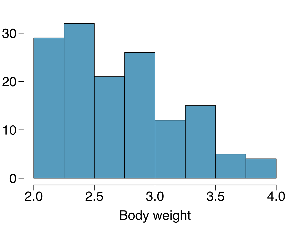
Cat weights. The histogram shown below represents the weights (in kg) of 47 female and 97 male cats.
(a) What fraction of these cats weigh less than 2.5 kg?
(b) What fraction of these cats weigh between 2.5 and 2.75 kg?
(c) What fraction of these cats weigh between 2.75 and 3.5 kg?
Answer (4 parts)
Approximate answers are OK.
.
.
.
3.39 §3.R source ↗
Grade distributions. Each row in the table below is a proposed grade distribution for a class. Identify each as a valid or invalid probability distribution, and explain your reasoning.
| Grades | |||||
| A | B | C | D | F | |
| (a) | 0.3 | 0.3 | 0.3 | 0.2 | 0.1 |
| (b) | 0 | 0 | 1 | 0 | 0 |
| (c) | 0.3 | 0.3 | 0.3 | 0 | 0 |
| (d) | 0.3 | 0.5 | 0.2 | 0.1 | -0.1 |
| (e) | 0.2 | 0.4 | 0.2 | 0.1 | 0.1 |
| (f) | 0 | -0.1 | 1.1 | 0 | 0 |
Answer (6 parts)
Invalid. Sum is greater than 1.
Valid. Probabilities are between 0 and 1, and they sum to 1. In this class, every student gets a C.
Invalid. Sum is less than 1.
Invalid. There is a negative probability.
Valid. Probabilities are between 0 and 1, and they sum to 1.
Invalid. There is a negative probability.
3.41 §3.R source ↗
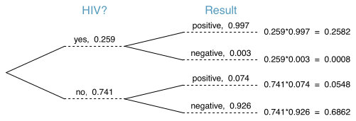
HIV in Swaziland. Swaziland has the highest HIV prevalence in the world: 25.9% of this country’s population is infected with HIV. The ELISA test is one of the first and most accurate tests for HIV. For those who carry HIV, the ELISA test is 99.7% accurate. For those who do not carry HIV, the test is 92.6% accurate. If an individual from Swaziland has tested positive, what is the probability that he carries HIV?
Answer
0.8247.
3.43 §3.R source ↗
Cost of breakfast. Sally gets a cup of coffee and a muffin every day for breakfast from one of the many coffee shops in her neighborhood. She picks a coffee shop each morning at random and independently of previous days. The average price of a cup of coffee is $1.40 with a standard deviation of 30¢ ($0.30), the average price of a muffin is $2.50 with a standard deviation of 15¢, and the two prices are independent of each other.
What is the mean and standard deviation of the amount she spends on breakfast daily?
What is the mean and standard deviation of the amount she spends on breakfast weekly (7 days)?
Answer (2 parts)
E = $3.90. SD = $0.34.
E = $27.30. SD = $0.89.
3.45 §3.R source ↗
Variance of a mean, Part I. Suppose we have independent observations and from a distribution with mean and standard deviation . What is the variance of the mean of the two values: ?
Answer
3.47 §3.R source ↗
Variance of a mean, Part III. Suppose we have independent observations , , ..., from a distribution with mean and standard deviation . What is the variance of the mean of these values: ?
Answer
(there are of these terms)
Loading chapter 4…
Exercises and answers are adapted from OpenIntro Statistics by David Diez, Mine Çetinkaya-Rundel and Christopher D Barr, which is free to read and download, and are used under the CC BY-SA 3.0 licence. They are taken from the book’s LaTeX source and set for the web, so they may differ slightly from the printed page. This adaptation is released under the same licence and is neither affiliated with nor endorsed by Diez, Çetinkaya-Rundel and Barr or OpenIntro.