Every problem in the chapter beside the book’s answer, a chapter at a time as you scroll.
Chapter 8: Introduction to linear regression
31 problems · 38 figuresGuided Practice 8.3 §8.1 source ↗
If a model underestimates an observation, will the residual be positive or negative? What about if it overestimates the observation?
Answer
If a model underestimates an observation, then the model estimate is below the actual. The residual, which is the actual observation value minus the model estimate, must then be positive. The opposite is true when the model overestimates the observation: the residual is negative.
Guided Practice 8.4 §8.1 source ↗
Compute the residuals for the “” observation and the “” observation in the figure using the linear relationship .
Answer
() First compute the predicted value based on the model:
Then the residual is given by
This was close to the earlier estimate of 7.
() . , close to the estimate of -4.
Guided Practice 8.6 §8.1 source ↗
No straight line is a good fit for the data sets represented in Figure 8.10. Try drawing nonlinear curves on each plot. Once you create a curve for each, describe what is important in your fit.
Answer
We’ll leave it to you to draw the lines. In general, the lines you draw should be close to most points and reflect overall trends in the data.
8.1 §8.1 source ↗
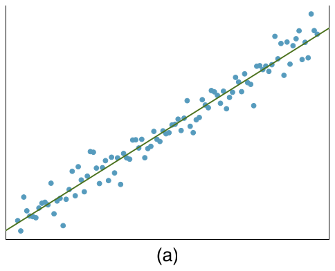
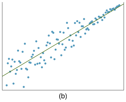
Visualize the residuals. The scatterplots shown below each have a superimposed regression line. If we were to construct a residual plot (residuals versus ) for each, describe what those plots would look like.
Answer (2 parts)
The residual plot will show randomly distributed residuals around 0. The variance is also approximately constant.
The residuals will show a fan shape, with higher variability for smaller . There will also be many points on the right above the line. There is trouble with the model being fit here.
8.3 §8.1 source ↗
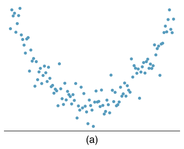
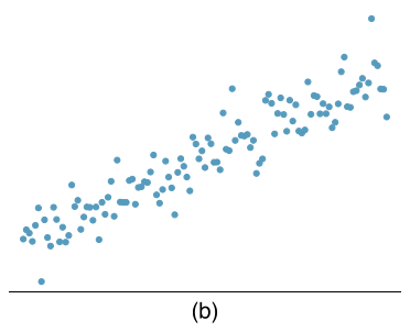
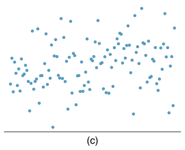
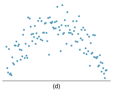
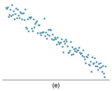
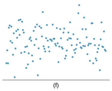
Identify relationships, Part I. For each of the six plots, identify the strength of the relationship (e.g. weak, moderate, or strong) in the data and whether fitting a linear model would be reasonable.
Answer (6 parts)
Strong relationship, but a straight line would not fit the data.
Strong relationship, and a linear fit would be reasonable.
Weak relationship, and trying a linear fit would be reasonable.
Moderate relationship, but a straight line would not fit the data.
Strong relationship, and a linear fit would be reasonable.
Weak relationship, and trying a linear fit would be reasonable.
8.5 §8.1 source ↗
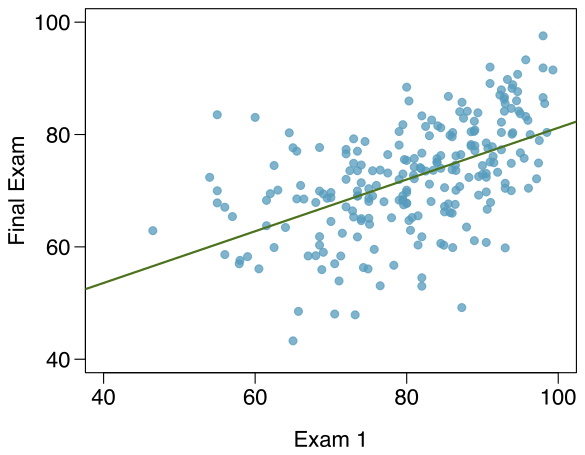
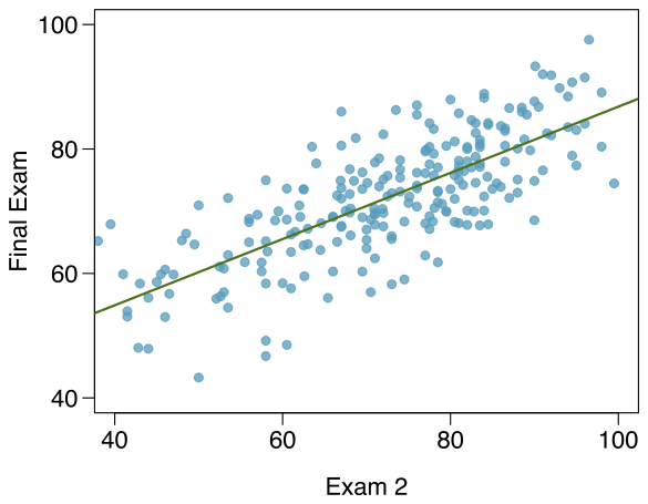
Exams and grades. The two scatterplots below show the relationship between final and mid-semester exam grades recorded during several years for a Statistics course at a university.
Based on these graphs, which of the two exams has the strongest correlation with the final exam grade? Explain.
Can you think of a reason why the correlation between the exam you chose in part (a) and the final exam is higher?
Answer (2 parts)
Exam 2 since there is less of a scatter in the plot of final exam grade versus exam 2. Notice that the relationship between Exam 1 and the Final Exam appears to be slightly nonlinear.
Exam 2 and the final are relatively close to each other chronologically, or Exam 2 may be cumulative so has greater similarities in material to the final exam. Answers may vary.
8.7 §8.1 source ↗
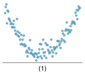
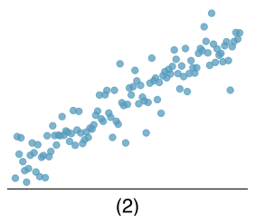
Match the correlation, Part I. Match each correlation to the corresponding scatterplot.
(a)
(b)
(c)
(d)
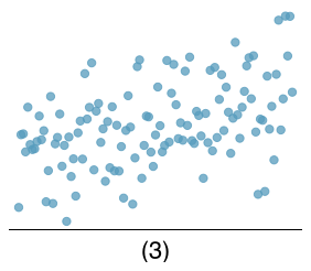
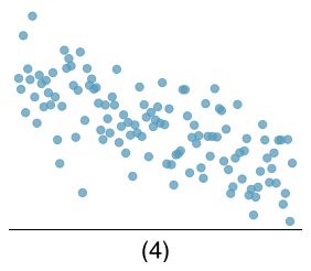
Answer (4 parts)
(4).
(3).
(1).
(2).
8.9 §8.1 source ↗
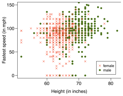
Speed and height. 1,302 UCLA students were asked to fill out a survey where they were asked about their height, fastest speed they have ever driven, and gender. The scatterplot on the left displays the relationship between height and fastest speed, and the scatterplot on the right displays the breakdown by gender in this relationship.
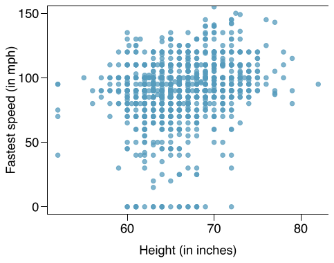
Describe the relationship between height and fastest speed.
Why do you think these variables are positively associated?
What role does gender play in the relationship between height and fastest driving speed?
Answer (3 parts)
The relationship is positive, weak, and possibly linear. However, there do appear to be some anomalous observations along the left where several students have the same height that is notably far from the cloud of the other points. Additionally, there are many students who appear not to have driven a car, and they are represented by a set of points along the bottom of the scatterplot.
There is no obvious explanation why simply being tall should lead a person to drive faster. However, one confounding factor is gender. Males tend to be taller than females on average, and personal experiences (anecdotal) may suggest they drive faster. If we were to follow-up on this suspicion, we would find that sociological studies confirm this suspicion.
Males are taller on average and they drive faster. The gender variable is indeed an important confounding variable.
8.11 §8.1 source ↗
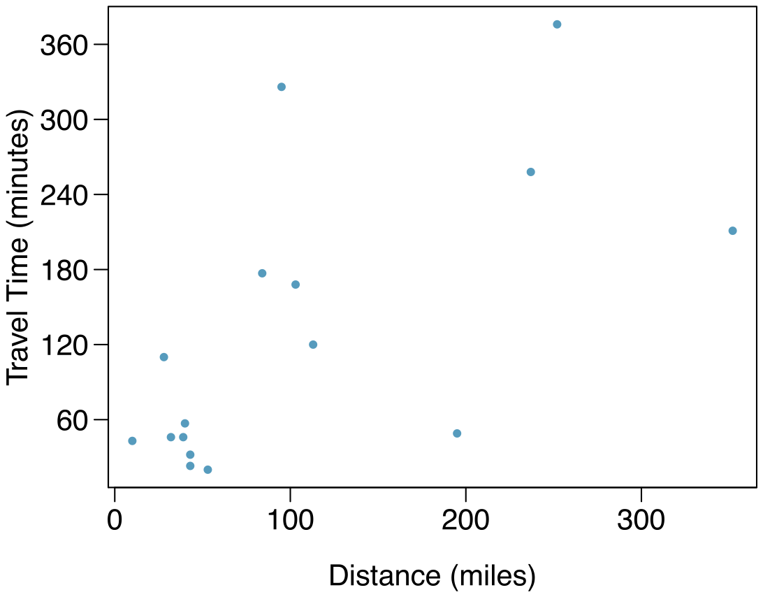
The Coast Starlight, Part I. The Coast Starlight Amtrak train runs from Seattle to Los Angeles. The scatterplot below displays the distance between each stop (in miles) and the amount of time it takes to travel from one stop to another (in minutes).
(a) Describe the relationship between distance and travel time.
(b) How would the relationship change if travel time was instead measured in hours, and distance was instead measured in kilometers?
(c) The correlation between travel time (in miles) and distance (in minutes) is . Suppose we had instead measured travel time in hours and measured distance in kilometers (km). What would be the correlation in these different units?
Answer (3 parts)
There is a somewhat weak, positive, possibly linear relationship between the distance traveled and travel time. There is clustering near the lower left corner that we should take special note of.
Changing the units will not change the form, direction or strength of the relationship between the two variables. If longer distances measured in miles are associated with longer travel time measured in minutes, longer distances measured in kilometers will be associated with longer travel time measured in hours.
Changing units doesn’t affect correlation: .
8.13 §8.1 source ↗
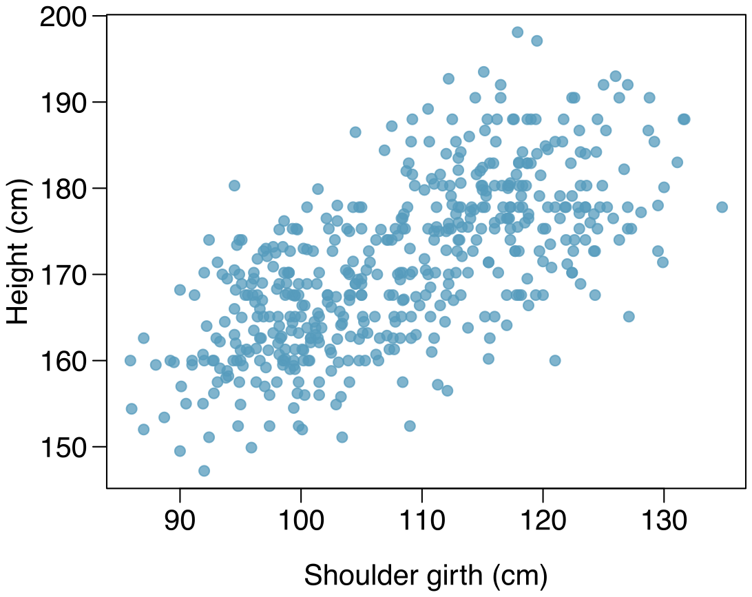
Body measurements, Part I. Researchers studying anthropometry collected body girth measurements and skeletal diameter measurements, as well as age, weight, height and gender for 507 physically active individuals. The scatterplot below shows the relationship between height and shoulder girth (over deltoid muscles), both measured in centimeters.
(a) Describe the relationship between shoulder girth and height.
(b) How would the relationship change if shoulder girth was measured in inches while the units of height remained in centimeters?
Answer (2 parts)
There is a moderate, positive, and linear relationship between shoulder girth and height.
Changing the units, even if just for one of the variables, will not change the form, direction or strength of the relationship between the two variables.
8.15 §8.1 source ↗
Correlation, Part I. What would be the correlation between the ages of husbands and wives if men always married woman who were
3 years younger than themselves?
2 years older than themselves?
half as old as themselves?
Answer (4 parts)
In each part, we can write the husband ages as a linear function of the wife ages.
.
.
.
Since the slopes are positive and these are perfect linear relationships, the correlation will be exactly 1 in all three parts. An alternative way to gain insight into this solution is to create a mock data set, e.g. 5 women aged 26, 27, 28, 29, and 30, then find the husband ages for each wife in each part and create a scatterplot.
Guided Practice 8.7 §8.2 source ↗
Is the correlation positive or negative in Figure 8.11?
Answer
Larger family incomes are associated with lower amounts of aid, so the correlation will be negative. Using a computer, the correlation can be computed: -0.499.
Guided Practice 8.8 §8.2 source ↗
Should we have concerns about applying least squares regression to the Elmhurst data in Figure 8.11?
Answer
The trend appears to be linear, the data fall around the line with no obvious outliers, the variance is roughly constant. These are also not time series observations. Least squares regression can be applied to these data.
Guided Practice 8.9 §8.2 source ↗
Using the summary statistics in Figure 8.13, compute the slope for the regression line of gift aid against family income.
| Family Income () | Gift Aid () | |
| mean | ||
| sd | ||
Answer
Compute the slope using the summary statistics from Figure 8.13:
| Family Income () | Gift Aid () | |
| mean | ||
| sd | ||
Guided Practice 8.15 §8.2 source ↗
If a linear model has a very strong negative relationship with a correlation of -0.97, how much of the variation in the response is explained by the explanatory variable?
Answer
About or 94% of the variation is explained by the linear model.
8.17 §8.2 source ↗
Units of regression. Consider a regression predicting weight (kg) from height (cm) for a sample of adult males. What are the units of the correlation coefficient, the intercept, and the slope?
Answer
Correlation: no units. Intercept: kg. Slope: kg/cm.
8.19 §8.2 source ↗
Over-under, Part I. Suppose we fit a regression line to predict the shelf life of an apple based on its weight. For a particular apple, we predict the shelf life to be 4.6 days. The apple’s residual is -0.6 days. Did we over or under estimate the shelf-life of the apple? Explain your reasoning.
Answer
Over-estimate. Since the residual is calculated as , a negative residual means that the predicted value is higher than the observed value.
8.21 §8.2 source ↗
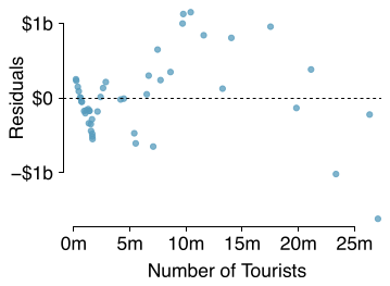
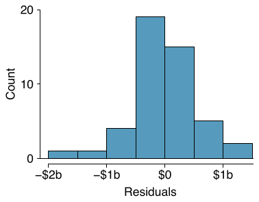
Tourism spending. The Association of Turkish Travel Agencies reports the number of foreign tourists visiting Turkey and tourist spending by year. Three plots are provided: scatterplot showing the relationship between these two variables along with the least squares fit, residuals plot, and histogram of residuals.
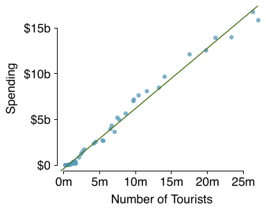
Describe the relationship between number of tourists and spending.
What are the explanatory and response variables?
Why might we want to fit a regression line to these data?
Do the data meet the conditions required for fitting a least squares line? In addition to the scatterplot, use the residual plot and histogram to answer this question.
Answer (4 parts)
There is a positive, very strong, linear association between the number of tourists and spending.
Explanatory: number of tourists (in thousands). Response: spending (in millions of US dollars).
We can predict spending for a given number of tourists using a regression line. This may be useful information for determining how much the country may want to spend in advertising abroad, or to forecast expected revenues from tourism.
Even though the relationship appears linear in the scatterplot, the residual plot actually shows a nonlinear relationship. This is not a contradiction: residual plots can show divergences from linearity that can be difficult to see in a scatterplot. A simple linear model is inadequate for modeling these data. It is also important to consider that these data are observed sequentially, which means there may be a hidden structure not evident in the current plots but that is important to consider.
8.23 §8.2 source ↗
The Coast Starlight, Part II. Exercise 8.11 introduces data on the Coast Starlight Amtrak train that runs from Seattle to Los Angeles. The mean travel time from one stop to the next on the Coast Starlight is 129 mins, with a standard deviation of 113 minutes. The mean distance traveled from one stop to the next is 108 miles with a standard deviation of 99 miles. The correlation between travel time and distance is 0.636.
Write the equation of the regression line for predicting travel time.
Interpret the slope and the intercept in this context.
Calculate of the regression line for predicting travel time from distance traveled for the Coast Starlight, and interpret in the context of the application.
The distance between Santa Barbara and Los Angeles is 103 miles. Use the model to estimate the time it takes for the Starlight to travel between these two cities.
It actually takes the Coast Starlight about 168 mins to travel from Santa Barbara to Los Angeles. Calculate the residual and explain the meaning of this residual value.
Suppose Amtrak is considering adding a stop to the Coast Starlight 500 miles away from Los Angeles. Would it be appropriate to use this linear model to predict the travel time from Los Angeles to this point?
The Coast Starlight, Part I. The Coast Starlight Amtrak train runs from Seattle to Los Angeles. The scatterplot below displays the distance between each stop (in miles) and the amount of time it takes to travel from one stop to another (in minutes).
(a) Describe the relationship between distance and travel time.
(b) How would the relationship change if travel time was instead measured in hours, and distance was instead measured in kilometers?
(c) The correlation between travel time (in miles) and distance (in minutes) is . Suppose we had instead measured travel time in hours and measured distance in kilometers (km). What would be the correlation in these different units?
Answer. (a) There is a somewhat weak, positive, possibly linear relationship between the distance traveled and travel time. There is clustering near the lower left corner that we should take special note of. (b) Changing the units will not change the form, direction or strength of the relationship between the two variables. If longer distances measured in miles are associated with longer travel time measured in minutes, longer distances measured in kilometers will be associated with longer travel time measured in hours. (c) Changing units doesn’t affect correlation: .
Answer (6 parts)
First calculate the slope: . Next, make use of the fact that the regression line passes through the point : . Plug in , , and , and solve for : 51. Solution: .
: For each additional mile in distance, the model predicts an additional 0.726 minutes in travel time. : When the distance traveled is 0 miles, the travel time is expected to be 51 minutes. It does not make sense to have a travel distance of 0 miles in this context. Here, the -intercept serves only to adjust the height of the line and is meaningless by itself.
. About 40% of the variability in travel time is accounted for by the model, i.e. explained by the distance traveled.
minutes. (Note: we should be cautious in our predictions with this model since we have not yet evaluated whether it is a well-fit model.)
minutes. A positive residual means that the model underestimates the travel time.
No, this calculation would require extrapolation.
8.25 §8.2 source ↗
Murders and poverty, Part I. The following regression output is for predicting annual murders per million from percentage living in poverty in a random sample of 20 metropolitan areas.
| Estimate | Std. Error | t value | Pr(t) | |
| (Intercept) | -29.901 | 7.789 | -3.839 | 0.001 |
| poverty% | 2.559 | 0.390 | 6.562 | 0.000 |
(a) Write out the linear model.
(b) Interpret the intercept.
(c) Interpret the slope.
(d) Interpret .
(e) Calculate the correlation coefficient.
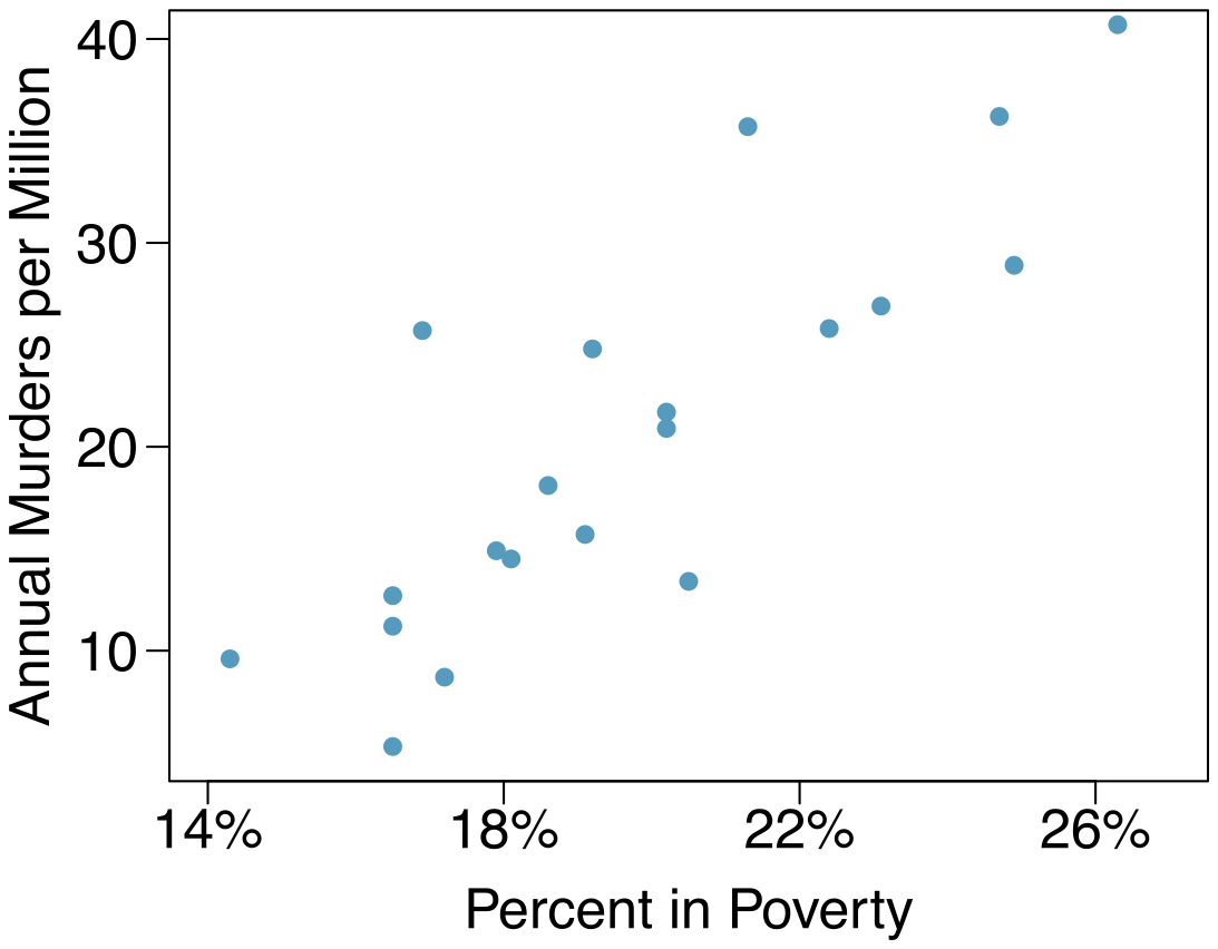
Answer (5 parts)
.
Expected murder rate in metropolitan areas with no poverty is -29. 901 per million. This is obviously not a meaningful value, it just serves to adjust the height of the regression line.
For each additional percentage increase in poverty, we expect murders per million to be higher on average by 2.559.
Poverty level explains 70.52% of the variability in murder rates in metropolitan areas.
.
8.27 §8.3 source ↗
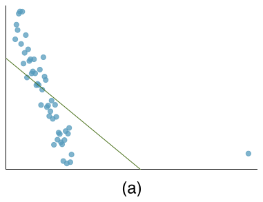
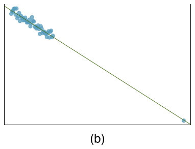
Outliers, Part I. Identify the outliers in the scatterplots shown below, and determine what type of outliers they are. Explain your reasoning.
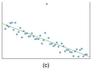
Answer (3 parts)
There is an outlier in the bottom right. Since it is far from the center of the data, it is a point with high leverage. It is also an influential point since, without that observation, the regression line would have a very different slope.
There is an outlier in the bottom right. Since it is far from the center of the data, it is a point with high leverage. However, it does not appear to be affecting the line much, so it is not an influential point.
The observation is in the center of the data (in the x-axis direction), so this point does not have high leverage. This means the point won’t have much effect on the slope of the line and so is not an influential point.
8.29 §8.3 source ↗
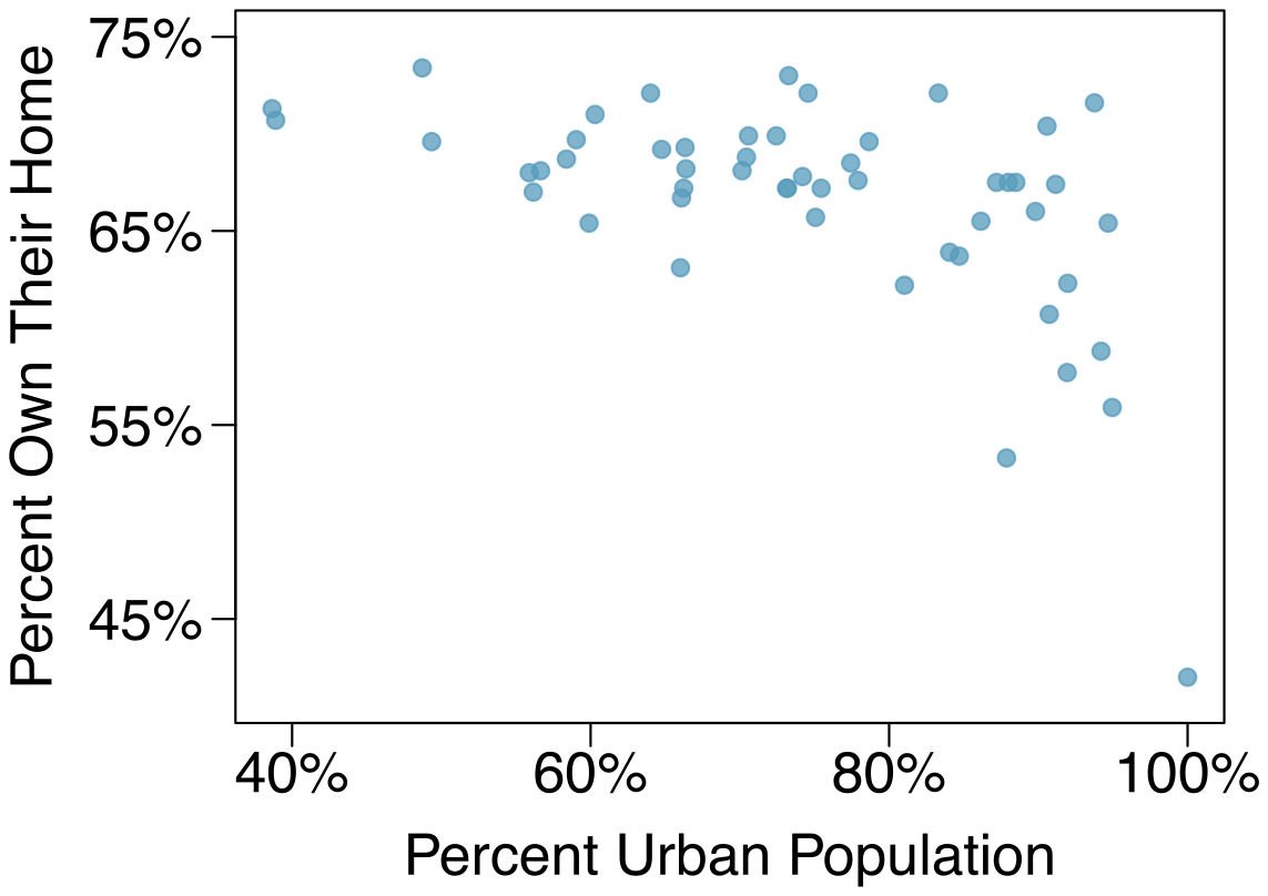
Urban homeowners, Part I. The scatterplot below shows the percent of families who own their home vs. the percent of the population living in urban areas. There are 52 observations, each corresponding to a state in the US. Puerto Rico and District of Columbia are also included.
(a) Describe the relationship between the percent of families who own their home and the percent of the population living in urban areas.
(b) The outlier at the bottom right corner is District of Columbia, where 100% of the population is considered urban. What type of an outlier is this observation?
Answer (2 parts)
There is a negative, moderate-to-strong, somewhat linear relationship between percent of families who own their home and the percent of the population living in urban areas in 2010. There is one outlier: a state where 100% of the population is urban. The variability in the percent of homeownership also increases as we move from left to right in the plot.
The outlier is located in the bottom right corner, horizontally far from the center of the other points, so it is a point with high leverage. It is an influential point since excluding this point from the analysis would greatly affect the slope of the regression line.
Guided Practice 8.18 §8.4 source ↗
The data for the Great Depression (1934 and 1938) were removed because the unemployment rate was 21% and 18%, respectively. Do you agree that they should be removed for this investigation? Why or why not?
Answer
We will provide two considerations. Each of these points would have very high leverage on any least-squares regression line, and years with such high unemployment may not help us understand what would happen in other years where the unemployment is only modestly high. On the other hand, these are exceptional cases, and we would be discarding important information if we exclude them from a final analysis.
Guided Practice 8.22 §8.4 source ↗
Figure 8.21 shows statistical software output from fitting the least squares regression line shown in Figure 8.15. Use this output to formally evaluate the following hypotheses.
: The true coefficient for family income is zero.
: The true coefficient for family income is not zero.
| Estimate | Std. Error | t value | Pr(t) | |
| (Intercept) | 24319.3 | 1291.5 | 18.83 | 0.0001 |
| family_income | -0.0431 | 0.0108 | -3.98 | 0.0002 |
Answer
We look in the second row corresponding to the family income variable. We see the point estimate of the slope of the line is -0.0431, the standard error of this estimate is 0.0108, and the -test statistic is . The p-value corresponds exactly to the two-sided test we are interested in: 0.0002. The p-value is so small that we reject the null hypothesis and conclude that family income and financial aid at Elmhurst College for freshman entering in the year 2011 are negatively correlated and the true slope parameter is indeed less than 0, just as we believed in Example 8.21.
Examine Figure 8.15, which relates the Elmhurst College aid and student family income. How sure are you that the slope is statistically significantly different from zero? That is, do you think a formal hypothesis test would reject the claim that the true slope of the line should be zero?
Answer. While the relationship between the variables is not perfect, there is an evident decreasing trend in the data. This suggests the hypothesis test will reject the null claim that the slope is zero.
8.31 §8.4 source ↗
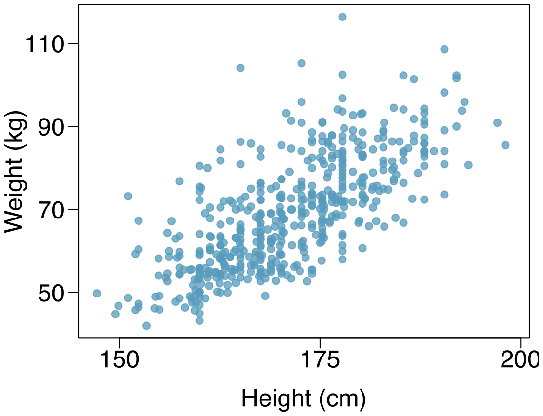
Body measurements, Part IV. The scatterplot and least squares summary below show the relationship between weight measured in kilograms and height measured in centimeters of 507 physically active individuals.
| Estimate | Std. Error | t value | Pr(t) | |
| (Intercept) | -105.0113 | 7.5394 | -13.93 | 0.0000 |
| height | 1.0176 | 0.0440 | 23.13 | 0.0000 |
Describe the relationship between height and weight.
Write the equation of the regression line. Interpret the slope and intercept in context.
Do the data provide strong evidence that an increase in height is associated with an increase in weight? State the null and alternative hypotheses, report the p-value, and state your conclusion.
The correlation coefficient for height and weight is 0.72. Calculate and interpret it in context.
Answer (4 parts)
The relationship is positive, moderate-to-strong, and linear. There are a few outliers but no points that appear to be influential.
.
Slope: For each additional centimeter in height, the model predicts the average weight to be 1.0176 additional kilograms (about 2.2 pounds).
Intercept: People who are 0 centimeters tall are expected to weigh - 105.0113 kilograms. This is obviously not possible. Here, the - intercept serves only to adjust the height of the line and is meaningless by itself.
: The true slope coefficient of height is zero ().
: The true slope coefficient of height is different than zero ().
The p-value for the two-sided alternative hypothesis () is incredibly small, so we reject . The data provide convincing evidence that height and weight are positively correlated. The true slope parameter is indeed greater than 0.
. Approximately 52% of the variability in weight can be explained by the height of individuals.
8.33 §8.4 source ↗
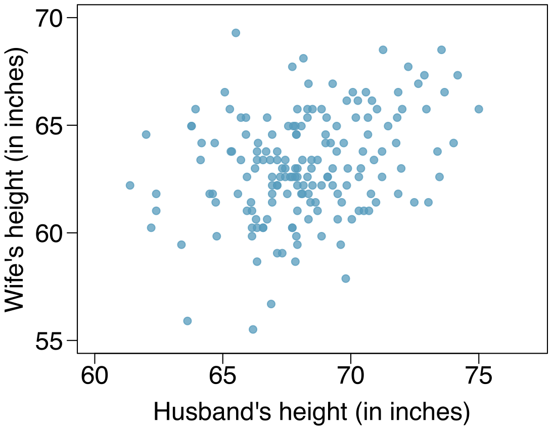
Husbands and wives, Part II. The scatterplot below summarizes husbands’ and wives’ heights in a random sample of 170 married couples in Britain, where both partners’ ages are below 65 years. Summary output of the least squares fit for predicting wife’s height from husband’s height is also provided in the table.
| Estimate | Std. Error | t value | Pr(t) | |
| (Intercept) | 43.5755 | 4.6842 | 9.30 | 0.0000 |
| height_ husband | 0.2863 | 0.0686 | 4.17 | 0.0000 |
Is there strong evidence that taller men marry taller women? State the hypotheses and include any information used to conduct the test.
Write the equation of the regression line for predicting wife’s height from husband’s height.
Interpret the slope and intercept in the context of the application.
Given that , what is the correlation of heights in this data set?
You meet a married man from Britain who is 5’9" (69 inches). What would you predict his wife’s height to be? How reliable is this prediction?
You meet another married man from Britain who is 6’7" (79 inches). Would it be wise to use the same linear model to predict his wife’s height? Why or why not?
Answer (6 parts)
: . : . The p-value, as reported in the table, is incredibly small and is smaller than 0.05, so we reject . The data provide convincing evidence that wives’ and husbands’ heights are positively correlated.
.
Slope: For each additional inch in husband’s height, the average wife’s height is expected to be an additional 0.2863 inches on average. Intercept: Men who are 0 inches tall are expected to have wives who are, on average, 43.5755 inches tall. The intercept here is meaningless, and it serves only to adjust the height of the line.
The slope is positive, so must also be positive. .
63.33. Since is low, the prediction based on this regression model is not very reliable.
No, we should avoid extrapolating.
8.35 §8.4 source ↗
Murders and poverty, Part II. Exercise 8.25 presents regression output from a model for predicting annual murders per million from percentage living in poverty based on a random sample of 20 metropolitan areas. The model output is also provided below.
| Estimate | Std. Error | t value | Pr(t) | |
| (Intercept) | -29.901 | 7.789 | -3.839 | 0.001 |
| poverty% | 2.559 | 0.390 | 6.562 | 0.000 |
What are the hypotheses for evaluating whether poverty percentage is a significant predictor of murder rate?
State the conclusion of the hypothesis test from part (a) in context of the data.
Calculate a 95% confidence interval for the slope of poverty percentage, and interpret it in context of the data.
Do your results from the hypothesis test and the confidence interval agree? Explain.
Murders and poverty, Part I. The following regression output is for predicting annual murders per million from percentage living in poverty in a random sample of 20 metropolitan areas.
| Estimate | Std. Error | t value | Pr(t) | |
| (Intercept) | -29.901 | 7.789 | -3.839 | 0.001 |
| poverty% | 2.559 | 0.390 | 6.562 | 0.000 |
(a) Write out the linear model.
(b) Interpret the intercept.
(c) Interpret the slope.
(d) Interpret .
(e) Calculate the correlation coefficient.
Answer. (a) . (b) Expected murder rate in metropolitan areas with no poverty is -29. 901 per million. This is obviously not a meaningful value, it just serves to adjust the height of the regression line. (c) For each additional percentage increase in poverty, we expect murders per million to be higher on average by 2.559. (d) Poverty level explains 70.52% of the variability in murder rates in metropolitan areas. (e) .
Answer (4 parts)
The p-value for this test is approximately 0, therefore we reject . The data provide convincing evidence that poverty percentage is a significant predictor of murder rate.
; ; For each percentage point poverty is higher, murder rate is expected to be higher on average by 1.74 to 3.378 per million.
Yes, we rejected and the confidence interval does not include 0.
8.37 §8.R source ↗
True / False. Determine if the following statements are true or false. If false, explain why.
A correlation coefficient of -0.90 indicates a stronger linear relationship than a correlation of 0.5.
Correlation is a measure of the association between any two variables.
Answer (2 parts)
True.
False, correlation is a measure of the linear association between any two numerical variables.
8.39 §8.R source ↗
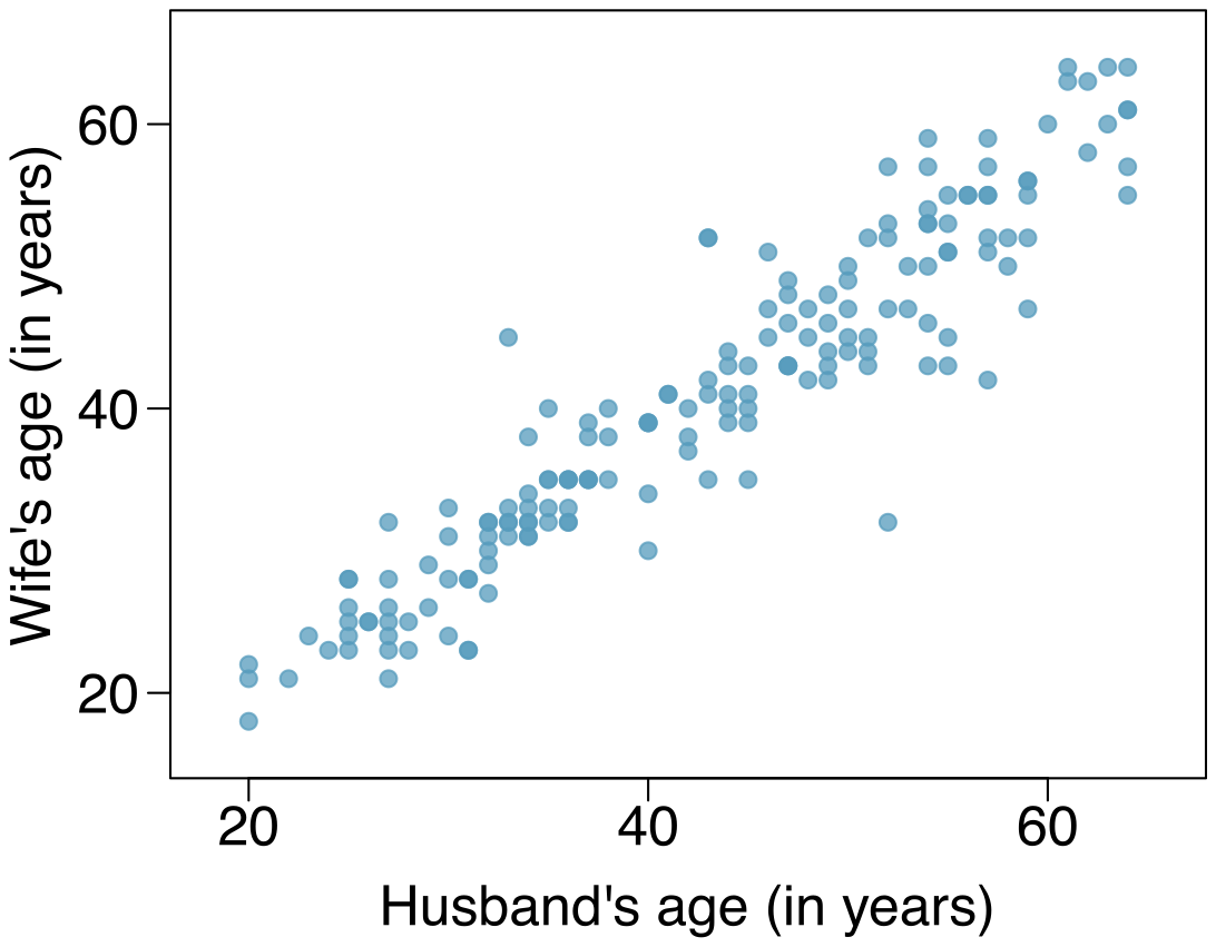
Husbands and wives, Part III. Exercise 8.33 presents a scatterplot displaying the relationship between husbands’ and wives’ ages in a random sample of 170 married couples in Britain, where both partners’ ages are below 65 years. Given below is summary output of the least squares fit for predicting wife’s age from husband’s age.
| Estimate | Std. Error | t value | Pr(t) | |
| (Intercept) | 1.5740 | 1.1501 | 1.37 | 0.1730 |
| age_ husband | 0.9112 | 0.0259 | 35.25 | 0.0000 |
We might wonder, is the age difference between husbands and wives consistent across ages? If this were the case, then the slope parameter would be . Use the information above to evaluate if there is strong evidence that the difference in husband and wife ages differs for different ages.
Write the equation of the regression line for predicting wife’s age from husband’s age.
Interpret the slope and intercept in context.
Given that , what is the correlation of ages in this data set?
You meet a married man from Britain who is 55 years old. What would you predict his wife’s age to be? How reliable is this prediction?
You meet another married man from Britain who is 85 years old. Would it be wise to use the same linear model to predict his wife’s age? Explain.
Husbands and wives, Part II. The scatterplot below summarizes husbands’ and wives’ heights in a random sample of 170 married couples in Britain, where both partners’ ages are below 65 years. Summary output of the least squares fit for predicting wife’s height from husband’s height is also provided in the table.
| Estimate | Std. Error | t value | Pr(t) | |
| (Intercept) | 43.5755 | 4.6842 | 9.30 | 0.0000 |
| height_ husband | 0.2863 | 0.0686 | 4.17 | 0.0000 |
(a) Is there strong evidence that taller men marry taller women? State the hypotheses and include any information used to conduct the test.
(b) Write the equation of the regression line for predicting wife’s height from husband’s height.
(c) Interpret the slope and intercept in the context of the application.
(d) Given that , what is the correlation of heights in this data set?
(e) You meet a married man from Britain who is 5’9" (69 inches). What would you predict his wife’s height to be? How reliable is this prediction?
(f) You meet another married man from Britain who is 6’7" (79 inches). Would it be wise to use the same linear model to predict his wife’s height? Why or why not?
Answer. (a) : . : . The p-value, as reported in the table, is incredibly small and is smaller than 0.05, so we reject . The data provide convincing evidence that wives’ and husbands’ heights are positively correlated.
(b) .
(c) Slope: For each additional inch in husband’s height, the average wife’s height is expected to be an additional 0.2863 inches on average. Intercept: Men who are 0 inches tall are expected to have wives who are, on average, 43.5755 inches tall. The intercept here is meaningless, and it serves only to adjust the height of the line.
(d) The slope is positive, so must also be positive. .
(e) 63.33. Since is low, the prediction based on this regression model is not very reliable.
(f) No, we should avoid extrapolating.
Answer (6 parts)
The point estimate and standard error are and . We can compute a T-score: . Using , the p-value is about 0.001, which is less than . That is, the data provide strong evidence that the average difference between husbands’ and wives’ ages has actually changed over time.
.
Slope: For each additional year in husband’s age, the model predicts an additional 0.9112 years in wife’s age. This means that wives’ ages tend to be lower for later ages, suggesting the average gap of husband and wife age is larger for older people. Intercept: Men who are 0 years old are expected to have wives who are on average 1.5740 years old. The intercept here is meaningless and serves only to adjust the height of the line.
. The regression of wives’ ages on husbands’ ages has a positive slope, so the correlation coefficient will be positive.
. Since is pretty high, the prediction based on this regression model is reliable.
No, we shouldn’t use the same model to predict an 85 year old man’s wife’s age. This would require extrapolation. The scatterplot from an earlier exercise shows that husbands in this data set are approximately 20 to 65 years old. The regression model may not be reasonable outside of this range.
8.41 §8.R source ↗
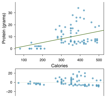
Nutrition at Starbucks, Part II. Exercise 8.22 introduced a data set on nutrition information on Starbucks food menu items. Based on the scatterplot and the residual plot provided, describe the relationship between the protein content and calories of these menu items, and determine if a simple linear model is appropriate to predict amount of protein from the number of calories.
Nutrition at Starbucks, Part I. The scatterplot below shows the relationship between the number of calories and amount of carbohydrates (in grams) Starbucks food menu items contain. Since Starbucks only lists the number of calories on the display items, we are interested in predicting the amount of carbs a menu item has based on its calorie content.
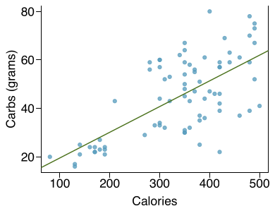
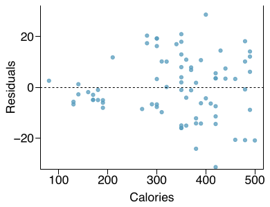
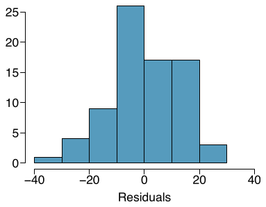
(a) Describe the relationship between number of calories and amount of carbohydrates (in grams) that Starbucks food menu items contain.
(b) In this scenario, what are the explanatory and response variables?
(c) Why might we want to fit a regression line to these data?
(d) Do these data meet the conditions required for fitting a least squares line?
Answer
There is an upwards trend. However, the variability is higher for higher calorie counts, and it looks like there might be two clusters of observations above and below the line on the right, so we should be cautious about fitting a linear model to these data.
8.43 §8.R source ↗
Match the correlation, Part III. Match each correlation to the corresponding scatterplot.
(a)
(b)
(c)
(d)
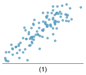
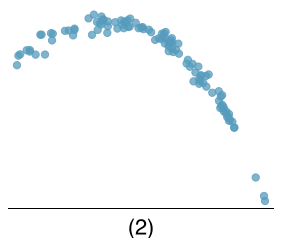
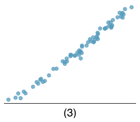
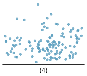
Answer (4 parts)
Loading chapter 9…
Exercises and answers are adapted from OpenIntro Statistics by David Diez, Mine Çetinkaya-Rundel and Christopher D Barr, which is free to read and download, and are used under the CC BY-SA 3.0 licence. They are taken from the book’s LaTeX source and set for the web, so they may differ slightly from the printed page. This adaptation is released under the same licence and is neither affiliated with nor endorsed by Diez, Çetinkaya-Rundel and Barr or OpenIntro.