Every problem in the chapter beside the book’s answer, a chapter at a time as you scroll.
Chapter 4: Distributions of random variables
57 problems · 9 figuresGuided Practice 4.1 §4.1 source ↗
Write down the short-hand for a normal distribution with
mean 5 and standard deviation 3,
mean -100 and standard deviation 10, and
mean 2 and standard deviation 9.
Answer (3 parts)
.
.
.
Guided Practice 4.3 §4.1 source ↗
Use Tom’s ACT score, 24, along with the ACT mean and standard deviation to find his Z-score.
Answer
Guided Practice 4.4 §4.1 source ↗
Let represent a random variable from , and suppose we observe .
Find the Z-score of .
Use the Z-score to determine how many standard deviations above or below the mean falls.
Answer (2 parts)
Its Z-score is given by .
The observation is 1.095 standard deviations above the mean. We know it must be above the mean since is positive.
Guided Practice 4.5 §4.1 source ↗
Head lengths of brushtail possums follow a normal distribution with mean 92.6 mm and standard deviation 3.6 mm. Compute the Z-scores for possums with head lengths of 95.4 mm and 85.8 mm.
Answer
For mm: . For mm: .
Guided Practice 4.6 §4.1 source ↗
Which of the observations in Guided Practice 4.5 is more unusual?
Head lengths of brushtail possums follow a normal distribution with mean 92.6 mm and standard deviation 3.6 mm. Compute the Z-scores for possums with head lengths of 95.4 mm and 85.8 mm.
Answer. For mm: . For mm: .
Answer
Because the absolute value of Z-score for the second observation is larger than that of the first, the second observation has a more unusual head length.
Guided Practice 4.8 §4.1 source ↗
If the probability of Shannon scoring at least 1190 is 0.3264, then what is the probability she scores less than 1190? Draw the normal curve representing this exercise, shading the lower region instead of the upper one.
Answer
We found this probability in Example 4.7: 0.6736.
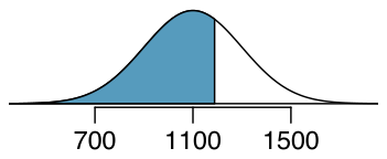
Shannon is a randomly selected SAT taker, and nothing is known about Shannon’s SAT aptitude. What is the probability Shannon scores at least 1190 on her SATs?
Answer. First, always draw and label a picture of the normal distribution. (Drawings need not be exact to be useful.) We are interested in the chance she scores above 1190, so we shade this upper tail:
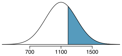
The picture shows the mean and the values at 2 standard deviations above and below the mean. The simplest way to find the shaded area under the curve makes use of the Z-score of the cutoff value. With , , and the cutoff value , the Z-score is computed as
Using statistical software (or another preferred method), we can find the area left of as 0.6736. To find the area above , we compute one minus the area of the lower tail:
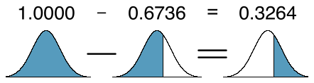
The probability Shannon scores at least 1190 on the SAT is 0.3264.
Guided Practice 4.10 §4.1 source ↗
Use the results of Example 4.9 to compute the proportion of SAT takers who did better than Edward. Also draw a new picture.
Edward earned a 1030 on his SAT. What is his percentile?
Answer. First, a picture is needed. Edward’s percentile is the proportion of people who do not get as high as a 1030. These are the scores to the left of 1030.
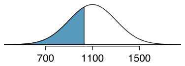
Identifying the mean , the standard deviation , and the cutoff for the tail area makes it easy to compute the Z-score:
Using statistical software, we get a tail area of 0.3632. Edward is at the percentile.
Answer
If Edward did better than 36% of SAT takers, then about 64% must have done better than him.
Guided Practice 4.11 §4.1 source ↗
Stuart earned an SAT score of 1500. Draw a picture for each part.
What is his percentile?
What percent of SAT takers did better than Stuart?
Answer (3 parts)
We leave the drawings to you.
.
.
Guided Practice 4.12 §4.1 source ↗
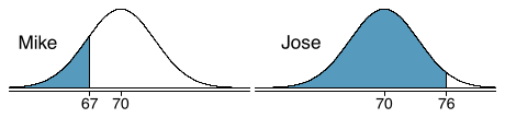
Mike is 5’7” and Jose is 6’4”, and they both live in the US.
What is Mike’s height percentile?
What is Jose’s height percentile?
Also draw one picture for each part.
Answer (3 parts)
First put the heights into inches: 67 and 76 inches. Figures are shown below.
.
.
Guided Practice 4.15 §4.1 source ↗
The SAT scores follow .
What is the percentile for SAT scores?
What is the percentile for SAT scores?
Answer (3 parts)
Short answers:
SAT score.
SAT score.
Guided Practice 4.16 §4.1 source ↗
Adult male heights follow ””.
What is the probability that a randomly selected male adult is at least 6’2” (74 inches)?
What is the probability that a male adult is shorter than 5’9” (69 inches)?
Answer (3 parts)
Short answers:
, then subtract this value from 1 to get 0.1131.
.
Guided Practice 4.18 §4.1 source ↗
SAT scores follow . What percent of SAT takers get between 1100 and 1400?
Answer
This is an abbreviated solution. (Be sure to draw a figure!) First find the percent who get below 1100 and the percent that get above 1400: (area below), (area above). Final answer: .
Guided Practice 4.19 §4.1 source ↗
Adult male heights follow ””. What percent of adult males are between 5’5” and 5’7”?
Answer
5’5” is 65 inches (). 5’7” is 67 inches (). Numerical solution: , i.e. 11.71%.
Guided Practice 4.20 §4.1 source ↗
Use software, a calculator, or a probability table to confirm that about 68%, 95%, and 99.7% of observations fall within 1, 2, and 3, standard deviations of the mean in the normal distribution, respectively. For instance, first find the area that falls between and , which should have an area of about 0.68. Similarly there should be an area of about 0.95 between and .
Answer
First draw the pictures. Using software, we get 0.6827 within 1 standard deviation, 0.9545 within 2 standard deviations, and 0.9973 within 3 standard deviations.
Guided Practice 4.21 §4.1 source ↗
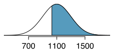
SAT scores closely follow the normal model with mean and standard deviation .
About what percent of test takers score 700 to 1500?
What percent score between 1100 and 1500?
Answer (2 parts)
700 and 1500 represent two standard deviations below and above the mean, which means about 95% of test takers will score between 700 and 1500.
We found that 700 to 1500 represents about 95% of test takers. These test takers would be evenly split by the center of the distribution, 1100, so of all test takers score between 1100 and 1500.
4.1 §4.1 source ↗
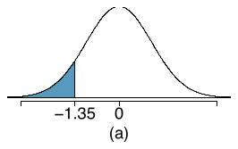
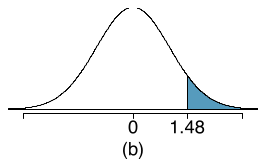
Area under the curve, Part I. What percent of a standard normal distribution is found in each region? Be sure to draw a graph.
Answer (4 parts)
8.85%.
6.94%.
58.86%.
4.56%.
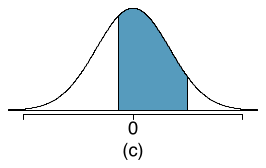
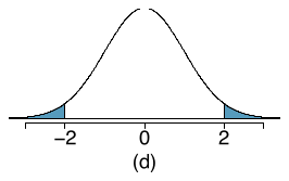
4.3 §4.1 source ↗
GRE scores, Part I. Sophia who took the Graduate Record Examination (GRE) scored 160 on the Verbal Reasoning section and 157 on the Quantitative Reasoning section. The mean score for Verbal Reasoning section for all test takers was 151 with a standard deviation of 7, and the mean score for the Quantitative Reasoning was 153 with a standard deviation of 7.67. Suppose that both distributions are nearly normal.
Write down the short-hand for these two normal distributions.
What is Sophia’s Z-score on the Verbal Reasoning section? On the Quantitative Reasoning section? Draw a standard normal distribution curve and mark these two Z-scores.
What do these Z-scores tell you?
Relative to others, which section did she do better on?
Find her percentile scores for the two exams.
What percent of the test takers did better than her on the Verbal Reasoning section? On the Quantitative Reasoning section?
Explain why simply comparing raw scores from the two sections could lead to an incorrect conclusion as to which section a student did better on.
If the distributions of the scores on these exams are not nearly normal, would your answers to parts (b) - (f) change? Explain your reasoning.
Answer (8 parts)
Verbal: , Quant: .
, .
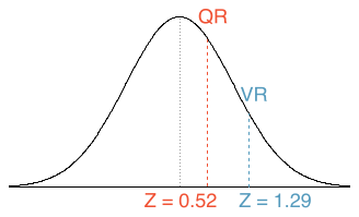
She scored 1.29 standard deviations above the mean on the Verbal Reasoning section and 0.52 standard deviations above the mean on the Quantitative Reasoning section.
She did better on the Verbal Reasoning section since her Z-score on that section was higher.
, .
did better than her on VR, and did better than her on QR.
We cannot compare the raw scores since they are on different scales. Comparing her percentile scores is more appropriate when comparing her performance to others.
Answer to part (b) would not change as Z-scores can be calculated for distributions that are not normal. However, we could not answer parts (d)-(f) since we cannot use the normal probability table to calculate probabilities and percentiles without a normal model.
4.5 §4.1 source ↗
GRE scores, Part II. In Exercise 4.3 we saw two distributions for GRE scores: for the verbal part of the exam and for the quantitative part. Use this information to compute each of the following:
The score of a student who scored in the percentile on the Quantitative Reasoning section.
The score of a student who scored worse than 70% of the test takers in the Verbal Reasoning section.
GRE scores, Part I. Sophia who took the Graduate Record Examination (GRE) scored 160 on the Verbal Reasoning section and 157 on the Quantitative Reasoning section. The mean score for Verbal Reasoning section for all test takers was 151 with a standard deviation of 7, and the mean score for the Quantitative Reasoning was 153 with a standard deviation of 7.67. Suppose that both distributions are nearly normal.
(a) Write down the short-hand for these two normal distributions.
(b) What is Sophia’s Z-score on the Verbal Reasoning section? On the Quantitative Reasoning section? Draw a standard normal distribution curve and mark these two Z-scores.
(c) What do these Z-scores tell you?
(d) Relative to others, which section did she do better on?
(e) Find her percentile scores for the two exams.
(f) What percent of the test takers did better than her on the Verbal Reasoning section? On the Quantitative Reasoning section?
(g) Explain why simply comparing raw scores from the two sections could lead to an incorrect conclusion as to which section a student did better on.
(h) If the distributions of the scores on these exams are not nearly normal, would your answers to parts (b) - (f) change? Explain your reasoning.
Answer. (a) Verbal: , Quant: . (b) , .
(c) She scored 1.29 standard deviations above the mean on the Verbal Reasoning section and 0.52 standard deviations above the mean on the Quantitative Reasoning section. (d) She did better on the Verbal Reasoning section since her Z-score on that section was higher. (e) , . (f) did better than her on VR, and did better than her on QR. (g) We cannot compare the raw scores since they are on different scales. Comparing her percentile scores is more appropriate when comparing her performance to others. (h) Answer to part (b) would not change as Z-scores can be calculated for distributions that are not normal. However, we could not answer parts (d)-(f) since we cannot use the normal probability table to calculate probabilities and percentiles without a normal model.
Answer (2 parts)
, which corresponds to approximately 159 on QR.
, which corresponds to approximately 147 on VR.
4.7 §4.1 source ↗
LA weather, Part I. The average daily high temperature in June in LA is 77F with a standard deviation of 5F. Suppose that the temperatures in June closely follow a normal distribution.
What is the probability of observing an 83F temperature or higher in LA during a randomly chosen day in June?
How cool are the coldest 10% of the days (days with lowest high temperature) during June in LA?
Answer (2 parts)
, .
F or colder.
4.9 §4.1 source ↗
LA weather, Part II. Exercise 4.7 states that average daily high temperature in June in LA is 77F with a standard deviation of 5F, and it can be assumed that they to follow a normal distribution. We use the following equation to convert F (Fahrenheit) to C (Celsius):
Write the probability model for the distribution of temperature in C in June in LA.
What is the probability of observing a 28C (which roughly corresponds to 83F) temperature or higher in June in LA? Calculate using the C model from part (a).
Did you get the same answer or different answers in part (b) of this question and part (a) of Exercise 4.7? Are you surprised? Explain.
Estimate the IQR of the temperatures (in C) in June in LA.
LA weather, Part I. The average daily high temperature in June in LA is 77F with a standard deviation of 5F. Suppose that the temperatures in June closely follow a normal distribution.
(a) What is the probability of observing an 83F temperature or higher in LA during a randomly chosen day in June?
(b) How cool are the coldest 10% of the days (days with lowest high temperature) during June in LA?
Answer. (a) , .
(b) F or colder.
Answer (4 parts)
.
, .
The answers are very close because only the units were changed. (The only reason why they differ at all because 28C is 82.4F, not precisely 83F.)
Since , we first need to find and and take the difference between the two. Remember that is the and is the percentile of a distribution. Q1 = 23.13, Q3 = 26.86, IQR = 26. 86 - 23.13 = 3.73.
Guided Practice 4.23 §4.2 source ↗
The probability that a particular case would not exceed their deductible is said to be 0.7. If we were to examine cases until we found one that where the person did not hit her deductible, how many cases should we expect to check?
Answer
We would expect to see about individuals to find the first success.
Guided Practice 4.25 §4.2 source ↗
Determine a more clever way to solve Example 4.24. Show that you get the same result.
What is the chance that we would find the first success within the first 3 cases?
Answer. This is the chance it is the first (), second (), or third () case is the first success, which are three disjoint outcomes. Because the individuals in the sample are randomly sampled from a large population, they are independent. We compute the probability of each case and add the separate results:
There is a probability of 0.973 that we would find a successful case within 3 cases.
Answer
First find the probability of the complement: no success in first 3 trials. Next, compute one minus this probability: no success in 3 trials.
Guided Practice 4.27 §4.2 source ↗
Using the results from Example 4.26, and , would it be appropriate to use the normal model to find what proportion of experiments would end in 3 or fewer trials?
Suppose a car insurer has determined that 88% of its drivers will not exceed their deductible in a given year. If someone at the company were to randomly draw driver files until they found one that had not exceeded their deductible, what is the expected number of drivers the insurance employee must check? What is the standard deviation of the number of driver files that must be drawn?
Answer. In this example, a success is again when someone will not exceed the insurance deductible, which has probability . The expected number of people to be checked is and the standard deviation is .
Answer
No. The geometric distribution is always right skewed and can never be well-approximated by the normal model.
4.11 §4.2 source ↗
Is it Bernoulli? Determine if each trial can be considered an independent Bernoulli trial for the following situations.
Cards dealt in a hand of poker.
Outcome of each roll of a die.
Answer (2 parts)
No. The cards are not independent. For example, if the first card is an ace of clubs, that implies the second card cannot be an ace of clubs. Additionally, there are many possible categories, which would need to be simplified.
No. There are six events under consideration. The Bernoulli distribution allows for only two events or categories. Note that rolling a die could be a Bernoulli trial if we simplify to two events, e.g. rolling a 6 and not rolling a 6, though specifying such details would be necessary.
4.13 §4.2 source ↗
Eye color, Part I. A husband and wife both have brown eyes but carry genes that make it possible for their children to have brown eyes (probability 0.75), blue eyes (0.125), or green eyes (0.125).
What is the probability the first blue-eyed child they have is their third child? Assume that the eye colors of the children are independent of each other.
On average, how many children would such a pair of parents have before having a blue-eyed child? What is the standard deviation of the number of children they would expect to have until the first blue-eyed child?
Answer (2 parts)
.
, .
4.15 §4.2 source ↗
Bernoulli, the mean. Use the probability rules from Section 3.4 to derive the mean of a Bernoulli random variable, i.e. a random variable that takes value 1 with probability and value 0 with probability . That is, compute the expected value of a generic Bernoulli random variable.
Answer
If is the probability of a success, then the mean of a Bernoulli random variable is given by
Guided Practice 4.29 §4.3 source ↗
Verify that the scenario where Brittany is the only one to exceed the deductible has probability .
Answer
.
Guided Practice 4.31 §4.3 source ↗
If we randomly sampled 40 case files from the insurance agency discussed earlier, how many of the cases would you expect to not have exceeded the deductible in a given year? What is the standard deviation of the number that would not have exceeded the deductible?
Answer
We are asked to determine the expected number (the mean) and the standard deviation, both of which can be directly computed from the formulas: and . Because very roughly 95% of observations fall within 2 standard deviations of the mean (see Section 2.1.4), we would probably observe at least 22 but fewer than 34 individuals in our sample who would not exceed the deductible.
Guided Practice 4.32 §4.3 source ↗
The probability that a random smoker will develop a severe lung condition in his or her lifetime is about . If you have 4 friends who smoke, are the conditions for the binomial model satisfied?
Answer
One possible answer: if the friends know each other, then the independence assumption is probably not satisfied. For example, acquaintances may have similar smoking habits, or those friends might make a pact to quit together.
Guided Practice 4.33 §4.3 source ↗
Suppose these four friends do not know each other and we can treat them as if they were a random sample from the population. Is the binomial model appropriate? What is the probability that
1. None of them will develop a severe lung condition?
2. One will develop a severe lung condition?
3. That no more than one will develop a severe lung condition?
Answer (4 parts)
To check if the binomial model is appropriate, we must verify the conditions. (i) Since we are supposing we can treat the friends as a random sample, they are independent. (ii) We have a fixed number of trials (). (iii) Each outcome is a success or failure. (iv) The probability of a success is the same for each trials since the individuals are like a random sample ( if we say a “success” is someone getting a lung condition, a morbid choice). Compute parts
and
using the binomial formula: , . Note: . Part
can be computed as the sum of parts (a) and (b): . That is, there is about a 65% chance that no more than one of your four smoking friends will develop a severe lung condition.
Guided Practice 4.34 §4.3 source ↗
What is the probability that at least 2 of your 4 smoking friends will develop a severe lung condition in their lifetimes?
Answer
The complement (no more than one will develop a severe lung condition) as computed in Guided Practice 4.33 as 0.6517, so we compute one minus this value: 0.3483.
Suppose these four friends do not know each other and we can treat them as if they were a random sample from the population. Is the binomial model appropriate? What is the probability that
1. None of them will develop a severe lung condition?
2. One will develop a severe lung condition?
3. That no more than one will develop a severe lung condition?
Answer. To check if the binomial model is appropriate, we must verify the conditions. (i) Since we are supposing we can treat the friends as a random sample, they are independent. (ii) We have a fixed number of trials (). (iii) Each outcome is a success or failure. (iv) The probability of a success is the same for each trials since the individuals are like a random sample ( if we say a “success” is someone getting a lung condition, a morbid choice). Compute parts (a) and (b) using the binomial formula: , . Note: . Part (c) can be computed as the sum of parts (a) and (b): . That is, there is about a 65% chance that no more than one of your four smoking friends will develop a severe lung condition.
Guided Practice 4.35 §4.3 source ↗
Suppose you have 7 friends who are smokers and they can be treated as a random sample of smokers.
1. How many would you expect to develop a severe lung condition, i.e. what is the mean?
2. What is the probability that at most 2 of your 7 friends will develop a severe lung condition.
Answer (2 parts)
.
0, 1, or 2 develop severe lung condition .
Guided Practice 4.36 §4.3 source ↗
Why is it true that and for any number ?
Answer
Frame these expressions into words. How many different ways are there to arrange 0 successes and failures in trials? (1 way.) How many different ways are there to arrange successes and 0 failures in trials? (1 way.)
Guided Practice 4.37 §4.3 source ↗
How many ways can you arrange one success and failures in trials? How many ways can you arrange successes and one failure in trials?
Answer
One success and failures: there are exactly unique places we can put the success, so there are ways to arrange one success and failures. A similar argument is used for the second question. Mathematically, we show these results by verifying the following two equations:
Guided Practice 4.39 §4.3 source ↗
Here we consider the binomial model when the probability of a success is . Figure 4.9 shows four hollow histograms for simulated samples from the binomial distribution using four different sample sizes: . What happens to the shape of the distributions as the sample size increases? What distribution does the last hollow histogram resemble?
Answer
The distribution is transformed from a blocky and skewed distribution into one that rather resembles the normal distribution in last hollow histogram.
Guided Practice 4.41 §4.3 source ↗
Use the normal model to estimate the probability of observing 42 or fewer smokers. Your answer should be approximately equal to the solution of Example 4.38: 0.0054.
Approximately 15% of the US population smokes cigarettes. A local government believed their community had a lower smoker rate and commissioned a survey of 400 randomly selected individuals. The survey found that only 42 of the 400 participants smoke cigarettes. If the true proportion of smokers in the community was really 15%, what is the probability of observing 42 or fewer smokers in a sample of 400 people?
Answer. We leave the usual verification that the four conditions for the binomial model are valid as an exercise.
The question posed is equivalent to asking, what is the probability of observing , 1, 2, ..., or 42 smokers in a sample of when ? We can compute these 43 different probabilities and add them together to find the answer:
If the true proportion of smokers in the community is , then the probability of observing 42 or fewer smokers in a sample of is 0.0054.
Answer
Compute the Z-score first: . The corresponding left tail area is 0.0059.
4.17 §4.3 source ↗
Underage drinking, Part I. Data collected by the Substance Abuse and Mental Health Services Administration (SAMSHA) suggests that 69.7% of 18-20 year olds consumed alcoholic beverages in any given year.
Suppose a random sample of ten 18-20 year olds is taken. Is the use of the binomial distribution appropriate for calculating the probability that exactly six consumed alcoholic beverages? Explain.
Calculate the probability that exactly 6 out of 10 randomly sampled 18- 20 year olds consumed an alcoholic drink.
What is the probability that exactly four out of ten 18-20 year olds have not consumed an alcoholic beverage?
What is the probability that at most 2 out of 5 randomly sampled 18-20 year olds have consumed alcoholic beverages?
What is the probability that at least 1 out of 5 randomly sampled 18-20 year olds have consumed alcoholic beverages?
Answer (5 parts)
Binomial conditions are met: (1) Independent trials: In a random sample, whether or not one 18-20 year old has consumed alcohol does not depend on whether or not another one has. (2) Fixed number of trials: . (3) Only two outcomes at each trial: Consumed or did not consume alcohol. (4) Probability of a success is the same for each trial: .
0.203.
0.203.
0.167.
0.997.
4.19 §4.3 source ↗
Underage drinking, Part II. We learned in Exercise 4.17 that about 70% of 18-20 year olds consumed alcoholic beverages in any given year. We now consider a random sample of fifty 18-20 year olds.
How many people would you expect to have consumed alcoholic beverages? And with what standard deviation?
Would you be surprised if there were 45 or more people who have consumed alcoholic beverages?
What is the probability that 45 or more people in this sample have consumed alcoholic beverages? How does this probability relate to your answer to part (b)?
Underage drinking, Part I. Data collected by the Substance Abuse and Mental Health Services Administration (SAMSHA) suggests that 69.7% of 18-20 year olds consumed alcoholic beverages in any given year.
(a) Suppose a random sample of ten 18-20 year olds is taken. Is the use of the binomial distribution appropriate for calculating the probability that exactly six consumed alcoholic beverages? Explain.
(b) Calculate the probability that exactly 6 out of 10 randomly sampled 18- 20 year olds consumed an alcoholic drink.
(c) What is the probability that exactly four out of ten 18-20 year olds have not consumed an alcoholic beverage?
(d) What is the probability that at most 2 out of 5 randomly sampled 18-20 year olds have consumed alcoholic beverages?
(e) What is the probability that at least 1 out of 5 randomly sampled 18-20 year olds have consumed alcoholic beverages?
Answer. (a) Binomial conditions are met: (1) Independent trials: In a random sample, whether or not one 18-20 year old has consumed alcohol does not depend on whether or not another one has. (2) Fixed number of trials: . (3) Only two outcomes at each trial: Consumed or did not consume alcohol. (4) Probability of a success is the same for each trial: . (b) 0.203. (c) 0.203. (d) 0.167. (e) 0.997.
Answer (3 parts)
,
. 45 is more than 3 standard deviations away from the mean, we can assume that it is an unusual observation. Therefore yes, we would be surprised.
Using the normal approximation, 0.0010. With 0.5 correction, 0.0017.
4.21 §4.3 source ↗
Game of dreidel. A dreidel is a four-sided spinning top with the Hebrew letters nun, gimel, hei, and shin, one on each side. Each side is equally likely to come up in a single spin of the dreidel. Suppose you spin a dreidel three times. Calculate the probability of getting
(a) at least one nun?
(b) exactly 2 nuns?
(c) exactly 1 hei?
(d) at most 2 gimels?
Answer (4 parts)
.
0.1406.
0.4219.
.
4.23 §4.3 source ↗
Eye color, Part II. Exercise 4.13 introduces a husband and wife with brown eyes who have 0.75 probability of having children with brown eyes, 0.125 probability of having children with blue eyes, and 0.125 probability of having children with green eyes.
What is the probability that their first child will have green eyes and the second will not?
What is the probability that exactly one of their two children will have green eyes?
If they have six children, what is the probability that exactly two will have green eyes?
If they have six children, what is the probability that at least one will have green eyes?
What is the probability that the first green eyed child will be the child?
Would it be considered unusual if only 2 out of their 6 children had brown eyes?
Eye color, Part I. A husband and wife both have brown eyes but carry genes that make it possible for their children to have brown eyes (probability 0.75), blue eyes (0.125), or green eyes (0.125).
(a) What is the probability the first blue-eyed child they have is their third child? Assume that the eye colors of the children are independent of each other.
(b) On average, how many children would such a pair of parents have before having a blue-eyed child? What is the standard deviation of the number of children they would expect to have until the first blue-eyed child?
Answer. (a) . (b) , .
Answer (6 parts)
Geometric distribution: 0.109.
Binomial: 0.219.
Binomial: 0.137.
.
Geometric: 0.084.
Using a binomial distribution with and , we see that , , and . Since this is not within 2 SD, it may be considered unusual.
4.25 §4.3 source ↗
Exploring permutations. The formula for the number of ways to arrange objects is . This exercise walks you through the derivation of this formula for a couple of special cases.
A small company has five employees: Anna, Ben, Carl, Damian, and Eddy. There are five parking spots in a row at the company, none of which are assigned, and each day the employees pull into a random parking spot. That is, all possible orderings of the cars in the row of spots are equally likely.
On a given day, what is the probability that the employees park in alphabetical order?
If the alphabetical order has an equal chance of occurring relative to all other possible orderings, how many ways must there be to arrange the five cars?
Now consider a sample of 8 employees instead. How many possible ways are there to order these 8 employees’ cars?
Answer (3 parts)
.
Since the probabilities must add to 1, there must be possible orderings.
.
Guided Practice 4.43 §4.4 source ↗
Suppose Brian is very diligent in his attempts and he makes each 35 yard field goal with probability . Take a guess at how many attempts he would need before making his fourth kick.
Answer
One possible answer: since he is likely to make each field goal attempt, it will take him at least 4 attempts but probably not more than 6 or 7.
Guided Practice 4.45 §4.4 source ↗
Each sequence in Figure 4.11 has exactly two failures and four successes with the last attempt always being a success. If the probability of a success is , find the probability of the first sequence.
| Kick Attempt | |||||||
| 1 | 2 | 3 | 4 | 5 | 6 | ||
| 1 | |||||||
| 2 | |||||||
| 3 | |||||||
| 4 | |||||||
| 5 | |||||||
| 6 | |||||||
| 7 | |||||||
| 8 | |||||||
| 9 | |||||||
| 10 | |||||||
Answer
The first sequence: .
Guided Practice 4.47 §4.4 source ↗
The negative binomial distribution requires that each kick attempt by Brian is independent. Do you think it is reasonable to suggest that each of Brian’s kick attempts are independent?
Answer
Answers may vary. We cannot conclusively say they are or are not independent. However, many statistical reviews of athletic performance suggests such attempts are very nearly independent.
Guided Practice 4.48 §4.4 source ↗
Assume Brian’s kick attempts are independent. What is the probability that Brian will kick his fourth field goal within 5 attempts?
Answer
If his fourth field goal () is within five attempts, it either took him four or five tries ( or ). We have from earlier. Use the negative binomial distribution to compute the probability of tries and tries, then add those probabilities together:
Guided Practice 4.49 §4.4 source ↗
On 70% of days, a hospital admits at least one heart attack patient. On 30% of the days, no heart attack patients are admitted. Identify each case below as a binomial or negative binomial case, and compute the probability.
1. What is the probability the hospital will admit a heart attack patient on exactly three days this week?
2. What is the probability the second day with a heart attack patient will be the fourth day of the week?
3. What is the probability the fifth day of next month will be the first day with a heart attack patient?
Answer (4 parts)
In each part, .
The number of days is fixed, so this is binomial. The parameters are and : 0.097.
The last “success” (admitting a heart attack patient) is fixed to the last day, so we should apply the negative binomial distribution. The parameters are , : 0.132.
This problem is negative binomial with and : 0.006. Note that the negative binomial case when is the same as using the geometric distribution.
4.27 §4.4 source ↗
Rolling a die. Calculate the following probabilities and indicate which probability distribution model is appropriate in each case. You roll a fair die 5 times. What is the probability of rolling
the first 6 on the fifth roll?
exactly three 6s?
the third 6 on the fifth roll?
Answer (3 parts)
Geometric, 0.0804.
Binomial, 0.0322.
Negative binomial, 0.0193.
4.29 §4.4 source ↗
Sampling at school. For a sociology class project you are asked to conduct a survey on 20 students at your school. You decide to stand outside of your dorm’s cafeteria and conduct the survey on a random sample of 20 students leaving the cafeteria after dinner one evening. Your dorm is comprised of 45% males and 55% females.
Which probability model is most appropriate for calculating the probability that the person you survey is the female? Explain.
Compute the probability from part (a).
The three possible scenarios that lead to person you survey being the female are One common feature among these scenarios is that the last trial is always female. In the first three trials there are 2 males and 1 female. Use the binomial coefficient to confirm that there are 3 ways of ordering 2 males and 1 female.
Use the findings presented in part (c) to explain why the formula for the coefficient for the negative binomial is while the formula for the binomial coefficient is .
Answer (4 parts)
Negative binomial with and , where a success is defined here as a female student. The negative binomial setting is appropriate since the last trial is fixed but the order of the first 3 trials is unknown.
0.1838.
.
In the binomial model there are no restrictions on the outcome of the last trial. In the negative binomial model the last trial is fixed. Therefore we are interested in the number of ways of orderings of the other successes in the first trials.
4.31 §4.5 source ↗
Customers at a coffee shop. A coffee shop serves an average of 75 customers per hour during the morning rush.
Which distribution have we studied that is most appropriate for calculating the probability of a given number of customers arriving within one hour during this time of day?
What are the mean and the standard deviation of the number of customers this coffee shop serves in one hour during this time of day?
Would it be considered unusually low if only 60 customers showed up to this coffee shop in one hour during this time of day?
Calculate the probability that this coffee shop serves 70 customers in one hour during this time of day.
Answer (4 parts)
Poisson with .
, .
. Since 60 is within 2 standard deviations of the mean, it would not generally be considered unusual. Note that we often use this rule of thumb even when the normal model does not apply.
Using Poisson with : 0.0402.
4.33 §4.5 source ↗
How many cars show up? For Monday through Thursday when there isn’t a holiday, the average number of vehicles that visit a particular retailer between 2pm and 3pm each afternoon is 6.5, and the number of cars that show up on any given day follows a Poisson distribution.
What is the probability that exactly 5 cars will show up next Monday?
What is the probability that 0, 1, or 2 cars will show up next Monday between 2pm and 3pm?
There is an average of 11.7 people who visit during those same hours from vehicles. Is it likely that the number of people visiting by car during this hour is also Poisson? Explain.
Answer (3 parts)
The probability will come to (0.0430 if no rounding error).
The number of people per car is , meaning people are coming in small clusters. That is, if one person arrives, there’s a chance that they brought one or more other people in their vehicle. This means individuals (the people) are not independent, even if the car arrivals are independent, and this breaks a core assumption for the Poisson distribution. That is, the number of people visiting between 2pm and 3pm would not follow a Poisson distribution.
4.35 §4.R source ↗
Roulette winnings. In the game of roulette, a wheel is spun and you place bets on where it will stop. One popular bet is that it will stop on a red slot; such a bet has an 18/38 chance of winning. If it stops on red, you double the money you bet. If not, you lose the money you bet. Suppose you play 3 times, each time with a $1 bet. Let Y represent the total amount won or lost. Write a probability model for Y.
Answer
0 wins (-$3): 0.1458. 1 win (-$1): 0.3936. 2 wins (+$1): 0.3543. 3 wins (+$3): 0.1063.
4.37 §4.R source ↗
University admissions. Suppose a university announced that it admitted 2,500 students for the following year’s freshman class. However, the university has dorm room spots for only 1,786 freshman students. If there is a 70% chance that an admitted student will decide to accept the offer and attend this university, what is the approximate probability that the university will not have enough dormitory room spots for the freshman class?
Answer
Want to find the probability that there will be 1,787 or more enrollees. Using the normal approximation, with and , , and . With a 0.5 correction: 0.0559.
4.39 §4.R source ↗
Auto insurance premiums. Suppose a newspaper article states that the distribution of auto insurance premiums for residents of California is approximately normal with a mean of $1,650. The article also states that 25% of California residents pay more than $1,800.
What is the Z-score that corresponds to the top 25% (or the percentile) of the standard normal distribution?
What is the mean insurance cost? What is the cutoff for the 75th percentile?
Identify the standard deviation of insurance premiums in California.
Answer (3 parts)
.
, .
.
4.41 §4.R source ↗
Married women. The American Community Survey estimates that 47.1% of women ages 15 years and over are married.
We randomly select three women between these ages. What is the probability that the third woman selected is the only one who is married?
What is the probability that all three randomly selected women are married?
On average, how many women would you expect to sample before selecting a married woman? What is the standard deviation?
If the proportion of married women was actually 30%, how many women would you expect to sample before selecting a married woman? What is the standard deviation?
Based on your answers to parts (c) and (d), how does decreasing the probability of an event affect the mean and standard deviation of the wait time until success?
Answer (5 parts)
.
.
, .
, .
When is smaller, the event is rarer, meaning the expected number of trials before a success and the standard deviation of the waiting time are higher.
4.43 §4.R source ↗
Overweight baggage. Suppose weights of the checked baggage of airline passengers follow a nearly normal distribution with mean 45 pounds and standard deviation 3.2 pounds. Most airlines charge a fee for baggage that weigh in excess of 50 pounds. Determine what percent of airline passengers incur this fee.
Answer
, , i.e. 6%.
4.45 §4.R source ↗
Buying books on Ebay. Suppose you’re considering buying your expensive chemistry textbook on Ebay. Looking at past auctions suggests that the prices of this textbook follow an approximately normal distribution with mean $89 and standard deviation $15.
What is the probability that a randomly selected auction for this book closes at more than $100?
Ebay allows you to set your maximum bid price so that if someone outbids you on an auction you can automatically outbid them, up to the maximum bid price you set. If you are only bidding on one auction, what are the advantages and disadvantages of setting a bid price too high or too low? What if you are bidding on multiple auctions?
If you watched 10 auctions, roughly what percentile might you use for a maximum bid cutoff to be somewhat sure that you will win one of these ten auctions? Is it possible to find a cutoff point that will ensure that you win an auction?
If you are willing to track up to ten auctions closely, about what price might you use as your maximum bid price if you want to be somewhat sure that you will buy one of these ten books?
Answer (4 parts)
, .
If you are bidding on only one auction and set a low maximum bid price, someone will probably outbid you. If you set a high maximum bid price, you may win the auction but pay more than is necessary. If bidding on more than one auction, and you set your maximum bid price very low, you probably won’t win any of the auctions. However, if the maximum bid price is even modestly high, you are likely to win multiple auctions.
An answer roughly equal to the 10th percentile would be reasonable. Regrettably, no percentile cutoff point guarantees beyond any possible event that you win at least one auction. However, you may pick a higher percentile if you want to be more sure of winning an auction.
Answers will vary a little but should correspond to the answer in part (c). We use the 10 percentile: .
4.47 §4.R source ↗
Heights of 10 year olds, Part III. Heights of 10 year olds, regardless of gender, closely follow a normal distribution with mean 55 inches and standard deviation 6 inches.
What fraction of 10 year olds are taller than 76 inches?
If there are 2,000 10 year olds entering Six Flags Magic Mountain in a single day, then compute the expected number of 10 year olds who are at least 76 inches tall. (You may assume the heights of the 10-year olds are independent.)
Using the binomial distribution, compute the probability that 0 of the 2,000 10 year olds will be at least 76 inches tall.
The number of 10 year olds who enter Six Flags Magic Mountain and are at least 76 inches tall in a given day follows a Poisson distribution with mean equal to the value found in part (b). Use the Poisson distribution to identify the probability no 10 year old will enter the park who is 76 inches or taller.
Answer (4 parts)
, upper tail is 0.0002. (More precise value: 0.000233, but we’ll use 0.0002 for the calculations here.)
. We would expect about 0.4 10 year olds who are 76 inches or taller to show up.
.
.
Loading chapter 5…
Exercises and answers are adapted from OpenIntro Statistics by David Diez, Mine Çetinkaya-Rundel and Christopher D Barr, which is free to read and download, and are used under the CC BY-SA 3.0 licence. They are taken from the book’s LaTeX source and set for the web, so they may differ slightly from the printed page. This adaptation is released under the same licence and is neither affiliated with nor endorsed by Diez, Çetinkaya-Rundel and Barr or OpenIntro.