Content check — Statistics (OpenIntro), Chapter 9: Multiple and logistic regression

Every problem in the chapter beside the book’s answer, a chapter at a time as you scroll.

Chapter 9: Multiple and logistic regression

28 problems · 9 figures

Guided Practice 9.5 §9.1 source ↗

Compute the average interest rate for borrowers whose income source and amount are both verified.

Answer

When income_ver takes a value of verified, then the corresponding variable takes a value of 1 while the other ( ${𝚒𝚗𝚌𝚘𝚖𝚎_𝚟𝚎𝚛}_{source_only}$ ⁠) is 0:

$\begin{matrix} \hat{r a t e} & = 11.10 + 1.42 \times 0 + 3.25 \times 1 \\ = 14.35 \end{matrix}$

The average interest rate for these borrowers is 14.35%.

Guided Practice 9.6 §9.1 source ↗

Interpret the coefficients in the income_ver model.

Answer

Each of the coefficients gives the incremental interest rate for the corresponding level relative to the not level, which is the reference level. For example, for a borrower whose income source and amount have been verified, the model predicts that they will have a 3.25% higher interest rate than a borrower who has not had their income source or amount verified.

Guided Practice 9.7 §9.1 source ↗

How much larger of an interest rate would we expect for a borrower who has verified their income source and amount vs a borrower whose income source has only been verified?

Answer

Relative to the not category, the verified category has an interest rate of 3.25% higher, while the source_only category is only 1.42% higher. Thus, verified borrowers will tend to get an interest rate about $3.25 % - 1.42 % = 1.83 %$ higher than source_only borrowers.

Guided Practice 9.10 §9.1 source ↗

What does $β_{4}$ ⁠, the coefficient of variable credit_util, represent? What is the point estimate of $β_{4}$ ⁠?

Answer

$β_{4}$ represents the change in interest rate we would expect if someone’s credit utilization was 0 and went to 1, all other factors held even. The point estimate is $b_{4} = 4.90 %$ ⁠.

Guided Practice 9.13 §9.1 source ↗

The estimated value of the intercept is 1.925, and one might be tempted to make some interpretation of this coefficient, such as, it is the model’s predicted price when each of the variables take value zero: income source is not verified, the borrower has no debt (debt-to-income and credit utilization are zero), and so on. Is this reasonable? Is there any value gained by making this interpretation?

Answer

Many of the variables do take a value 0 for at least one data point, and for those variables, it is reasonable. However, one variable never takes a value of zero: term, which describes the length of the loan, in months. If term is set to zero, then the loan must be paid back immediately; the borrower must give the money back as soon as she receives it, which means it is not a real loan. Ultimately, the interpretation of the intercept in this setting is not insightful.

Guided Practice 9.14 §9.1 source ↗

The variance of the residuals for the model given in Guided Practice 9.9 is 18.53, and the variance of the total price in all the auctions is 25.01. Calculate $R^{2}$ for this model.

Guided Practice 9.9 in the book ↗

Write out the regression model using the point estimates from Figure 9.5. How many predictors are there in this model?

Answer. The fitted model for the interest rate is given by:

$\begin{matrix} \hat{𝚛𝚊𝚝𝚎} & = 1.925 + 0.975 \times {𝚒𝚗𝚌𝚘𝚖𝚎_𝚟𝚎𝚛}_{source_only} + 2.537 \times {𝚒𝚗𝚌𝚘𝚖𝚎_𝚟𝚎𝚛}_{verified} + 0.021 \times 𝚍𝚎𝚋𝚝_𝚝𝚘_𝚒𝚗𝚌𝚘𝚖𝚎 \\ + 4.896 \times 𝚌𝚛𝚎𝚍𝚒𝚝_𝚞𝚝𝚒𝚕 + 0.386 \times 𝚋𝚊𝚗𝚔𝚛𝚞𝚙𝚝𝚌𝚢 + 0.154 \times 𝚝𝚎𝚛𝚖 \\ + 0.028 \times {𝚒𝚜𝚜𝚞𝚎𝚍}_{Jan2018} - 0.040 \times {𝚒𝚜𝚜𝚞𝚎𝚍}_{Mar2018} + 0.228 \times 𝚌𝚛𝚎𝚍𝚒𝚝_𝚌𝚑𝚎𝚌𝚔𝚜 \end{matrix}$

If we count up the number of predictor coefficients, we get the effective number of predictors in the model: $k = 9$ ⁠. Notice that the issued categorical predictor counts as two, once for the two levels shown in the model. In general, a categorical predictor with $p$ different levels will be represented by $p - 1$ terms in a multiple regression model.

Answer

$R^{2} = 1 - \frac{18.53}{25.01} = 0.2591$ ⁠.

Guided Practice 9.15 §9.1 source ↗

There were $n = 10000$ auctions in the loans data set and $k = 9$ predictor variables in the model. Use $n$ ⁠, $k$ ⁠, and the variances from Guided Practice 9.14 to calculate $R_{a d j}^{2}$ for the interest rate model.

Guided Practice 9.14 in the book ↗

The variance of the residuals for the model given in Guided Practice 9.9 is 18.53, and the variance of the total price in all the auctions is 25.01. Calculate $R^{2}$ for this model.

Answer. $R^{2} = 1 - \frac{18.53}{25.01} = 0.2591$ ⁠.

Answer

$R_{a d j}^{2} =$ $1 -$ $\frac{18.53}{25.01} \times \frac{10000 - 1}{1000 - 9 - 1} =$ $0.2584$ ⁠. While the difference is very small, it will be important when we fine tune the model in the next section.

Guided Practice 9.16 §9.1 source ↗

Suppose you added another predictor to the model, but the variance of the errors $V a r (e_{i})$ didn’t go down. What would happen to the $R^{2}$ ⁠? What would happen to the adjusted $R^{2}$ ⁠?

Answer

The unadjusted $R^{2}$ would stay the same and the adjusted $R^{2}$ would go down.

9.1 §9.1 source ↗

Baby weights, Part I. The Child Health and Development Studies investigate a range of topics. One study considered all pregnancies between 1960 and 1967 among women in the Kaiser Foundation Health Plan in the San Francisco East Bay area. Here, we study the relationship between smoking and weight of the baby. The variable smoke is coded 1 if the mother is a smoker, and 0 if not. The summary table below shows the results of a linear regression model for predicting the average birth weight of babies, measured in ounces, based on the smoking status of the mother.

	Estimate	Std. Error	t value	Pr( $>$ $\|$ ⁠t⁠ $\|$ ⁠)
(Intercept)	123.05	0.65	189.60	0.0000
smoke	-8.94	1.03	-8.65	0.0000

The variability within the smokers and non-smokers are about equal and the distributions are symmetric. With these conditions satisfied, it is reasonable to apply the model. (Note that we don’t need to check linearity since the predictor has only two levels.)

(a)

Write the equation of the regression model.

(b)

Interpret the slope in this context, and calculate the predicted birth weight of babies born to smoker and non-smoker mothers.

(c)

Is there a statistically significant relationship between the average birth weight and smoking?

Answer (3 parts)

(a)

$\hat{b a b y_w e i g h t} =$ $123.05 -$ $8.94 \times s m o k e$

(b)

The estimated body weight of babies born to smoking mothers is 8.94 ounces lower than babies born to non-smoking mothers. Smoker: $123.05 - 8.94 \times 1 = 114.11$ ounces. Non-smoker: $123.05 - 8.94 \times 0 = 123.05$ ounces.

(c)

$H_{0}$ ⁠: $β_{1} = 0$ ⁠. $H_{A}$ ⁠: $β_{1} \neq 0$ ⁠. $T = - 8.65$ ⁠, and the p-value is approximately 0. Since the p-value is very small, we reject $H_{0}$ ⁠. The data provide strong evidence that the true slope parameter is different than 0 and that there is an association between birth weight and smoking. Furthermore, having rejected $H_{0}$ ⁠, we can conclude that smoking is associated with lower birth weights.

9.3 §9.1 source ↗

Exercise 9.1 in the book ↗

	Estimate	Std. Error	t value	Pr( $>$ $\|$ ⁠t⁠ $\|$ ⁠)
(Intercept)	123.05	0.65	189.60	0.0000
smoke	-8.94	1.03	-8.65	0.0000

(a) Write the equation of the regression model.

(b) Interpret the slope in this context, and calculate the predicted birth weight of babies born to smoker and non-smoker mothers.

Answer. (a) $\hat{b a b y_w e i g h t} =$ $123.05 -$ $8.94 \times s m o k e$ (b) The estimated body weight of babies born to smoking mothers is 8.94 ounces lower than babies born to non-smoking mothers. Smoker: $123.05 - 8.94 \times 1 = 114.11$ ounces. Non-smoker: $123.05 - 8.94 \times 0 = 123.05$ ounces. (c) $H_{0}$ ⁠: $β_{1} = 0$ ⁠. $H_{A}$ ⁠: $β_{1} \neq 0$ ⁠. $T = - 8.65$ ⁠, and the p-value is approximately 0. Since the p-value is very small, we reject $H_{0}$ ⁠. The data provide strong evidence that the true slope parameter is different than 0 and that there is an association between birth weight and smoking. Furthermore, having rejected $H_{0}$ ⁠, we can conclude that smoking is associated with lower birth weights.

Exercise 9.2 in the book ↗

Baby weights, Part II. Exercise 9.1 introduces a data set on birth weight of babies. Another variable we consider is parity, which is 1 if the child is the first born, and 0 otherwise. The summary table below shows the results of a linear regression model for predicting the average birth weight of babies, measured in ounces, from parity.

	Estimate	Std. Error	t value	Pr( $>$ $\|$ ⁠t⁠ $\|$ ⁠)
(Intercept)	120.07	0.60	199.94	0.0000
parity	-1.93	1.19	-1.62	0.1052

(a) Write the equation of the regression model.

(b) Interpret the slope in this context, and calculate the predicted birth weight of first borns and others.

Baby weights, Part III. We considered the variables smoke and parity, one at a time, in modeling birth weights of babies in Exercises 9.1 and 9.2. A more realistic approach to modeling infant weights is to consider all possibly related variables at once. Other variables of interest include length of pregnancy in days (gestation), mother’s age in years (age), mother’s height in inches (height), and mother’s pregnancy weight in pounds (weight). Below are three observations from this data set.

	bwt	gestation	parity	age	height	weight	smoke
1	120	284	0	27	62	100	0
2	113	282	0	33	64	135	0
$⋮$	$⋮$	$⋮$	$⋮$	$⋮$	$⋮$	$⋮$	$⋮$
1236	117	297	0	38	65	129	0

The summary table below shows the results of a regression model for predicting the average birth weight of babies based on all of the variables included in the data set.

	Estimate	Std. Error	t value	Pr( $>$ $\|$ ⁠t⁠ $\|$ ⁠)
(Intercept)	-80.41	14.35	-5.60	0.0000
gestation	0.44	0.03	15.26	0.0000
parity	-3.33	1.13	-2.95	0.0033
age	-0.01	0.09	-0.10	0.9170
height	1.15	0.21	5.63	0.0000
weight	0.05	0.03	1.99	0.0471
smoke	-8.40	0.95	-8.81	0.0000

(a)

Write the equation of the regression model that includes all of the variables.

(b)

Interpret the slopes of gestation and age in this context.

(c)

The coefficient for parity is different than in the linear model shown in Exercise 9.2. Why might there be a difference?

(d)

Calculate the residual for the first observation in the data set.

(e)

The variance of the residuals is 249.28, and the variance of the birth weights of all babies in the data set is 332.57. Calculate the $R^{2}$ and the adjusted $R^{2}$ ⁠. Note that there are 1,236 observations in the data set.

Answer (5 parts)

(a)

$\hat{b a b y_w e i g h t} =$ $-$ $80.41 +$ $0.44 \times g e s t a t i o n -$ $3.33 \times p a r i t y -$ $0.01 \times a g e +$ $1.15 \times h e i g h t +$ $0.05 \times w e i g h t -$ $8.40 \times s m o k e$ ⁠.

(b)

$β_{g e s t a t i o n}$ ⁠: The model predicts a 0.44 ounce increase in the birth weight of the baby for each additional day of pregnancy, all else held constant. $β_{a g e}$ ⁠: The model predicts a 0.01 ounce decrease in the birth weight of the baby for each additional year in mother’s age, all else held constant.

(c)

Parity might be correlated with one of the other variables in the model, which complicates model estimation.

(d)

$\hat{b a b y_w e i g h t} = 120.58$ ⁠. $e = 120 - 120.58 = - 0.58$ ⁠. The model over-predicts this baby’s birth weight.

(e)

$R^{2} = 0.2504$ ⁠. $R_{a d j}^{2} = 0.2468$ ⁠.

9.5 §9.1 source ↗

GPA. A survey of 55 Duke University students asked about their GPA, number of hours they study at night, number of nights they go out, and their gender. Summary output of the regression model is shown below. Note that male is coded as 1.

	Estimate	Std. Error	t value	Pr( $>$ $\|$ ⁠t⁠ $\|$ ⁠)
(Intercept)	3.45	0.35	9.85	0.00
studyweek	0.00	0.00	0.27	0.79
sleepnight	0.01	0.05	0.11	0.91
outnight	0.05	0.05	1.01	0.32
gender	-0.08	0.12	-0.68	0.50

(a)

Calculate a 95% confidence interval for the coefficient of gender in the model, and interpret it in the context of the data.

(b)

Would you expect a 95% confidence interval for the slope of the remaining variables to include 0? Explain

Answer (2 parts)

(a)

(-0.32, 0.16). We are 95% confident that male students on average have GPAs 0.32 points lower to 0.16 points higher than females when controlling for the other variables in the model.

(b)

Yes, since the p-value is larger than 0.05 in all cases (not including the intercept).

Guided Practice 9.20 §9.2 source ↗

Examine Figure 9.7 on page , which considers the model including all variables except the variable for the month the loan was issued. If we were using the p-value approach with backward elimination and we were considering this model, which of these variables would be up for elimination? Would we drop that variable, or would we keep it in the model?

Figure 9.7 in the book ↗


	Estimate	Std. Error	t value	Pr( $>$ $\|$ ⁠t⁠ $\|$ ⁠)

(Intercept)	1.9213	0.1982	9.69	$<$ ⁠0.0001
income_ver: source_only	0.9740	0.0991	9.83	$<$ ⁠0.0001
income_ver: verified	2.5355	0.1172	21.64	$<$ ⁠0.0001
debt_to_income	0.0211	0.0029	7.19	$<$ ⁠0.0001
credit_util	4.8958	0.1619	30.25	$<$ ⁠0.0001
bankruptcy	0.3869	0.1324	2.92	0.0035
term	0.1537	0.0039	38.97	$<$ ⁠0.0001
credit_checks	0.2283	0.0182	12.51	$<$ ⁠0.0001

$R_{a d j}^{2} = 0.25854$			$d f = 9992$

The fit for the regression model after dropping the issued variable.

Answer

The bankruptcy predictor is up for elimination since it has the largest p-value. However, since that p-value is smaller than 0.05, we would still keep it in the model.

9.7 §9.2 source ↗

Baby weights, Part IV. Exercise 9.3 considers a model that predicts a newborn’s weight using several predictors (gestation length, parity, age of mother, height of mother, weight of mother, smoking status of mother). The table below shows the adjusted R-squared for the full model as well as adjusted R-squared values for all models we evaluate in the first step of the backwards elimination process.

	Model	Adjusted $R^{2}$
1	Full model	0.2541
2	No gestation	0.1031
3	No parity	0.2492
4	No age	0.2547
5	No height	0.2311
6	No weight	0.2536
7	No smoking status	0.2072

Which, if any, variable should be removed from the model first?

Exercise 9.3 in the book ↗

	bwt	gestation	parity	age	height	weight	smoke
1	120	284	0	27	62	100	0
2	113	282	0	33	64	135	0
$⋮$	$⋮$	$⋮$	$⋮$	$⋮$	$⋮$	$⋮$	$⋮$
1236	117	297	0	38	65	129	0

The summary table below shows the results of a regression model for predicting the average birth weight of babies based on all of the variables included in the data set.

	Estimate	Std. Error	t value	Pr( $>$ $\|$ ⁠t⁠ $\|$ ⁠)
(Intercept)	-80.41	14.35	-5.60	0.0000
gestation	0.44	0.03	15.26	0.0000
parity	-3.33	1.13	-2.95	0.0033
age	-0.01	0.09	-0.10	0.9170
height	1.15	0.21	5.63	0.0000
weight	0.05	0.03	1.99	0.0471
smoke	-8.40	0.95	-8.81	0.0000

(a) Write the equation of the regression model that includes all of the variables.

(b) Interpret the slopes of gestation and age in this context.

(c) The coefficient for parity is different than in the linear model shown in Exercise 9.2. Why might there be a difference?

(d) Calculate the residual for the first observation in the data set.

(e) The variance of the residuals is 249.28, and the variance of the birth weights of all babies in the data set is 332.57. Calculate the $R^{2}$ and the adjusted $R^{2}$ ⁠. Note that there are 1,236 observations in the data set.

Answer. (a) $\hat{b a b y_w e i g h t} =$ $-$ $80.41 +$ $0.44 \times g e s t a t i o n -$ $3.33 \times p a r i t y -$ $0.01 \times a g e +$ $1.15 \times h e i g h t +$ $0.05 \times w e i g h t -$ $8.40 \times s m o k e$ ⁠. (b) $β_{g e s t a t i o n}$ ⁠: The model predicts a 0.44 ounce increase in the birth weight of the baby for each additional day of pregnancy, all else held constant. $β_{a g e}$ ⁠: The model predicts a 0.01 ounce decrease in the birth weight of the baby for each additional year in mother’s age, all else held constant. (c) Parity might be correlated with one of the other variables in the model, which complicates model estimation. (d) $\hat{b a b y_w e i g h t} = 120.58$ ⁠. $e = 120 - 120.58 = - 0.58$ ⁠. The model over-predicts this baby’s birth weight. (e) $R^{2} = 0.2504$ ⁠. $R_{a d j}^{2} = 0.2468$ ⁠.

Answer

Remove age.

9.9 §9.2 source ↗

Baby weights, Part V. Exercise 9.3 provides regression output for the full model (including all explanatory variables available in the data set) for predicting birth weight of babies. In this exercise we consider a forward-selection algorithm and add variables to the model one-at-a-time. The table below shows the p-value and adjusted $R^{2}$ of each model where we include only the corresponding predictor. Based on this table, which variable should be added to the model first?

variable	gestation	parity	age	height	weight	smoke
p-value	$2.2 \times 10^{- 16}$	0.1052	0.2375	$2.97 \times 10^{- 12}$	$8.2 \times 10^{- 8}$	$2.2 \times 10^{- 16}$
$R_{a d j}^{2}$	0.1657	0.0013	0.0003	0.0386	0.0229	0.0569

Exercise 9.3 in the book ↗

	bwt	gestation	parity	age	height	weight	smoke
1	120	284	0	27	62	100	0
2	113	282	0	33	64	135	0
$⋮$	$⋮$	$⋮$	$⋮$	$⋮$	$⋮$	$⋮$	$⋮$
1236	117	297	0	38	65	129	0

The summary table below shows the results of a regression model for predicting the average birth weight of babies based on all of the variables included in the data set.

	Estimate	Std. Error	t value	Pr( $>$ $\|$ ⁠t⁠ $\|$ ⁠)
(Intercept)	-80.41	14.35	-5.60	0.0000
gestation	0.44	0.03	15.26	0.0000
parity	-3.33	1.13	-2.95	0.0033
age	-0.01	0.09	-0.10	0.9170
height	1.15	0.21	5.63	0.0000
weight	0.05	0.03	1.99	0.0471
smoke	-8.40	0.95	-8.81	0.0000

(a) Write the equation of the regression model that includes all of the variables.

(b) Interpret the slopes of gestation and age in this context.

(c) The coefficient for parity is different than in the linear model shown in Exercise 9.2. Why might there be a difference?

(d) Calculate the residual for the first observation in the data set.

Answer

Based on the p-value alone, either gestation or smoke should be added to the model first. However, since the adjusted $R^{2}$ for the model with gestation is higher, it would be preferable to add gestation in the first step of the forward- selection algorithm. (Other explanations are possible. For instance, it would be reasonable to only use the adjusted $R^{2}$ ⁠.)

9.11 §9.2 source ↗

Movie lovers, Part I. Suppose a social scientist is interested in studying what makes audiences love or hate a movie. She collects a random sample of movies (genre, length, cast, director, budget, etc.) as well as a measure of the success of the movie (score on a film review aggregator website). If as part of her research she is interested in finding out which variables are significant predictors of movie success, what type of model selection method should she use?

Answer

She should use p-value selection since she is interested in finding out about significant predictors, not just optimizing predictions.

9.13 §9.3 source ↗

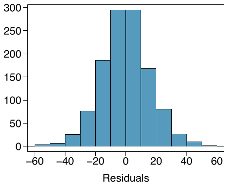
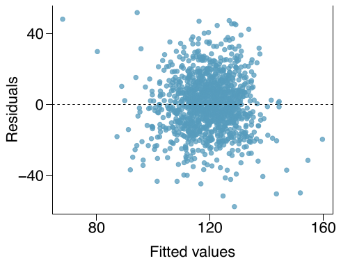
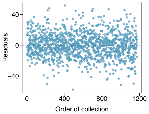
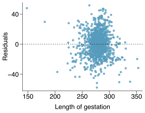
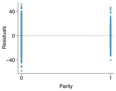
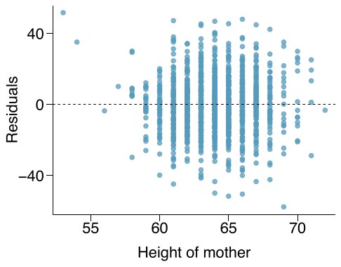
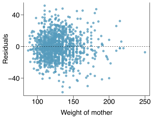
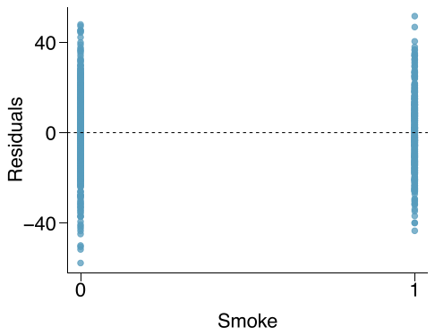
Baby weights, Part VI. Exercise 9.3 presents a regression model for predicting the average birth weight of babies based on length of gestation, parity, height, weight, and smoking status of the mother. Determine if the model assumptions are met using the plots below. If not, describe how to proceed with the analysis.

A histogram of residuals is shown, which has a bell-shaped distribution, is centered at 0, and has a standard deviation of about 12.

A scatterplot of ”residuals” (vertical axis) against ”fitted values”. The residuals does not show any pattern for different fitted values.

A scatterplot of ”residuals” (vertical axis) against ”order of collection”. The residuals does not show any pattern across the order of collection variable.

A scatterplot of ”residuals” (vertical axis) against ”length of gestation”. The residuals does not show any pattern for different lengths of gestation.

A scatterplot of ”residuals” (vertical axis) against ”parity”, which only takes values 0 and 1. The residuals does not show any apparent patterns across the values 0 and 1 of parity.

A scatterplot of ”residuals” (vertical axis) against ”height of mother”. The residuals does not show any pattern for different values of ”height of mother”.

A scatterplot of ”residuals” (vertical axis) against ”weight of mother”. The residuals does not show any pattern for different values of ”weight of mother”.

A scatterplot of ”residuals” (vertical axis) against ”smoke”, which only takes values 0 and 1. The residuals does not show any pattern for the 0 and 1 values of smoke.

Exercise 9.3 in the book ↗

	bwt	gestation	parity	age	height	weight	smoke
1	120	284	0	27	62	100	0
2	113	282	0	33	64	135	0
$⋮$	$⋮$	$⋮$	$⋮$	$⋮$	$⋮$	$⋮$	$⋮$
1236	117	297	0	38	65	129	0

The summary table below shows the results of a regression model for predicting the average birth weight of babies based on all of the variables included in the data set.

	Estimate	Std. Error	t value	Pr( $>$ $\|$ ⁠t⁠ $\|$ ⁠)
(Intercept)	-80.41	14.35	-5.60	0.0000
gestation	0.44	0.03	15.26	0.0000
parity	-3.33	1.13	-2.95	0.0033
age	-0.01	0.09	-0.10	0.9170
height	1.15	0.21	5.63	0.0000
weight	0.05	0.03	1.99	0.0471
smoke	-8.40	0.95	-8.81	0.0000

(a) Write the equation of the regression model that includes all of the variables.

(b) Interpret the slopes of gestation and age in this context.

(c) The coefficient for parity is different than in the linear model shown in Exercise 9.2. Why might there be a difference?

(d) Calculate the residual for the first observation in the data set.

Answer

Nearly normal residuals: With so many observations in the data set, we look for particularly extreme outliers in the histogram and do not see any. variability of residuals: The scatterplot of the residuals versus the fitted values does not show any overall structure. However, values that have very low or very high fitted values appear to also have somewhat larger outliers. In addition, the residuals do appear to have constant variability between the two parity and smoking status groups, though these items are relatively minor.
Independent residuals: The scatterplot of residuals versus the order of data collection shows a random scatter, suggesting that there is no apparent structures related to the order the data were collected.
Linear relationships between the response variable and numerical explanatory variables: The residuals vs. height and weight of mother are randomly distributed around 0. The residuals vs. length of gestation plot also does not show any clear or strong remaining structures, with the possible exception of very short or long gestations. The rest of the residuals do appear to be randomly distributed around 0.
All concerns raised here are relatively mild. There are some outliers, but there is so much data that the influence of such observations will be minor.

Guided Practice 9.21 §9.4 source ↗

We fit a linear regression model with the game’s condition as a predictor of auction price. Results of this model are summarized below:


	Estimate	Std. Error	t value	Pr( $>$ $\|$ ⁠t⁠ $\|$ ⁠)

(Intercept)	42.8711	0.8140	52.67	$<$ ⁠0.0001
cond_new	10.8996	1.2583	8.66	$<$ ⁠0.0001
			$d f = 139$

Write down the equation for the model, note whether the slope is statistically different from zero, and interpret the coefficient.

Answer

The equation for the line may be written as

$\begin{matrix} \hat{p r i c e} & = 42.87 + 10.90 \times c o n d_n e w \end{matrix}$

Examining the regression output in Guided Practice 9.21, we can see that the p-value for cond_new is very close to zero, indicating there is strong evidence that the coefficient is different from zero when using this simple one-variable model.

The cond_new is a two-level categorical variable that takes value 1 when the game is new and value 0 when the game is used. This means the 10.90 model coefficient predicts an extra $10.90 for those games that are new versus those that are used.

Guided Practice 9.22 §9.4 source ↗

Write out the model’s equation using the point estimates from Figure 9.15. How many predictors are there in this model?

Figure 9.15 in the book ↗


	Estimate	Std. Error	t value	Pr( $>$ $\|$ ⁠t⁠ $\|$ ⁠)

(Intercept)	36.2110	1.5140	23.92	$<$ ⁠0.0001
cond_new	5.1306	1.0511	4.88	$<$ ⁠0.0001
stock_photo	1.0803	1.0568	1.02	0.3085
duration	-0.0268	0.1904	-0.14	0.8882
wheels	7.2852	0.5547	13.13	$<$ ⁠0.0001
			$d f = 136$

Output for the regression model where price is the outcome and cond_new, stock_photo, duration, and wheels are the predictors.

Answer

$\hat{p r i c e} =$ $36.21 +$ $5.13 \times 𝚌𝚘𝚗𝚍_𝚗𝚎𝚠 +$ $1.08 \times 𝚜𝚝𝚘𝚌𝚔_𝚙𝚑𝚘𝚝𝚘 -$ $0.03 \times 𝚍𝚞𝚛𝚊𝚝𝚒𝚘𝚗 +$ $7.29 \times 𝚠𝚑𝚎𝚎𝚕𝚜$ ⁠, with the $k = 4$ predictors.

Guided Practice 9.23 §9.4 source ↗

What does $β_{4}$ ⁠, the coefficient of variable $x_{4}$ (Wii wheels), represent? What is the point estimate of $β_{4}$ ⁠?

Answer

It is the average difference in auction price for each additional Wii wheel included when holding the other variables constant. The point estimate is $b_{4} = 7.29$ ⁠.

Guided Practice 9.24 §9.4 source ↗

Compute the residual of the first observation in Figure 9.13 using the equation identified in Guided Practice 9.22.

Figure 9.13 in the book ↗

	price	cond_new	stock_photo	duration	wheels
1	51.55	1	1	3	1
2	37.04	0	1	7	1
$⋮$	$⋮$	$⋮$	$⋮$	$⋮$	$⋮$
140	38.76	0	0	7	0
141	54.51	1	1	1	2

Four observations from the mariokart data set.

Guided Practice 9.22 in the book ↗

Write out the model’s equation using the point estimates from Figure 9.15. How many predictors are there in this model?

Answer. $\hat{p r i c e} =$ $36.21 +$ $5.13 \times 𝚌𝚘𝚗𝚍_𝚗𝚎𝚠 +$ $1.08 \times 𝚜𝚝𝚘𝚌𝚔_𝚙𝚑𝚘𝚝𝚘 -$ $0.03 \times 𝚍𝚞𝚛𝚊𝚝𝚒𝚘𝚗 +$ $7.29 \times 𝚠𝚑𝚎𝚎𝚕𝚜$ ⁠, with the $k = 4$ predictors.

Answer

$e_{i} =$ $y_{i} -$ $\hat{y_{i}} =$ $51.55 -$ $49.62 =$ $1.93$ ⁠, where 49.62 was computed using the variables values from the observation and the equation identified in Guided Practice 9.22.

Guided Practice 9.22 in the book ↗

Write out the model’s equation using the point estimates from Figure 9.15. How many predictors are there in this model?

Guided Practice 9.27 §9.4 source ↗

In Example 9.26, we eliminated the duration variable, which resulted in a model with $R_{a d j}^{2} = 0.7128$ ⁠. Let’s look at if we would eliminate another variable from the model using backwards elimination:

Exclude `duration` and ...	`cond_new`	`stock_photo`	`wheels`
	$R_{a d j}^{2} = 0.6587$	$R_{a d j}^{2} = 0.7124$	$R_{a d j}^{2} = 0.3414$

Should we eliminate any additional variable, and if so, which variable should we eliminate?

Example 9.26 in the book ↗

Results corresponding to the full model for the mariokart data were shown in Figure 9.15. For this model, we consider what would happen if dropping each of the variables in the model:

Exclude ...	`cond_new`	`stock_photo`	`duration`	`wheels`
	$R_{a d j}^{2} = 0.6626$	$R_{a d j}^{2} = 0.7107$	$R_{a d j}^{2} = 0.7128$	$R_{a d j}^{2} = 0.3487$

For the full model, $R_{a d j}^{2} = 0.7108$ ⁠. How should we proceed under the backward elimination strategy?

Answer. The third model without duration has the highest $R_{a d j}^{2}$ of 0.7128, so we compare it to $R_{a d j}^{2}$ for the full model. Because eliminating duration leads to a model with a higher $R_{a d j}^{2}$ ⁠, we drop duration from the model.

Answer

Removing any of the three remaining variables would lead to a decrease in $R_{a d j}^{2}$ ⁠, so we should not remove any additional variables from the model after we removed duration.

Guided Practice 9.28 §9.4 source ↗

After eliminating the auction’s duration from the model, we are left with the following reduced model:

$\begin{matrix} \hat{p r i c e} & = 36.05 + 5.18 \times 𝚌𝚘𝚗𝚍_𝚗𝚎𝚠 + 1.12 \times 𝚜𝚝𝚘𝚌𝚔_𝚙𝚑𝚘𝚝𝚘 + 7.30 \times 𝚠𝚑𝚎𝚎𝚕𝚜 \end{matrix}$

How much would you predict for the total price for the Mario Kart game if it was used, used a stock photo, and included two wheels and put up for auction during the time period that the Mario Kart data were collected?

Answer

We would plug in 0 for cond_new 1 for stock_photo, and 2 for wheels into the equation, which would return $51.77, which is the total price we would expect for the auction.

Guided Practice 9.29 §9.4 source ↗

Would you be surprised if the seller from Guided Practice 9.28 didn’t get the exact price predicted?

Guided Practice 9.28 in the book ↗

After eliminating the auction’s duration from the model, we are left with the following reduced model:

$\begin{matrix} \hat{p r i c e} & = 36.05 + 5.18 \times 𝚌𝚘𝚗𝚍_𝚗𝚎𝚠 + 1.12 \times 𝚜𝚝𝚘𝚌𝚔_𝚙𝚑𝚘𝚝𝚘 + 7.30 \times 𝚠𝚑𝚎𝚎𝚕𝚜 \end{matrix}$

Answer. We would plug in 0 for cond_new 1 for stock_photo, and 2 for wheels into the equation, which would return $51.77, which is the total price we would expect for the auction.

Answer

No. The model provides the average auction price we would expect, and the price for one auction to the next will continue to vary a bit (but less than what our prediction would be without the model).

9.15 §9.5 source ↗

Figure 8.4 View it in the book ↗

The common brushtail possum of Australia.
—————————–

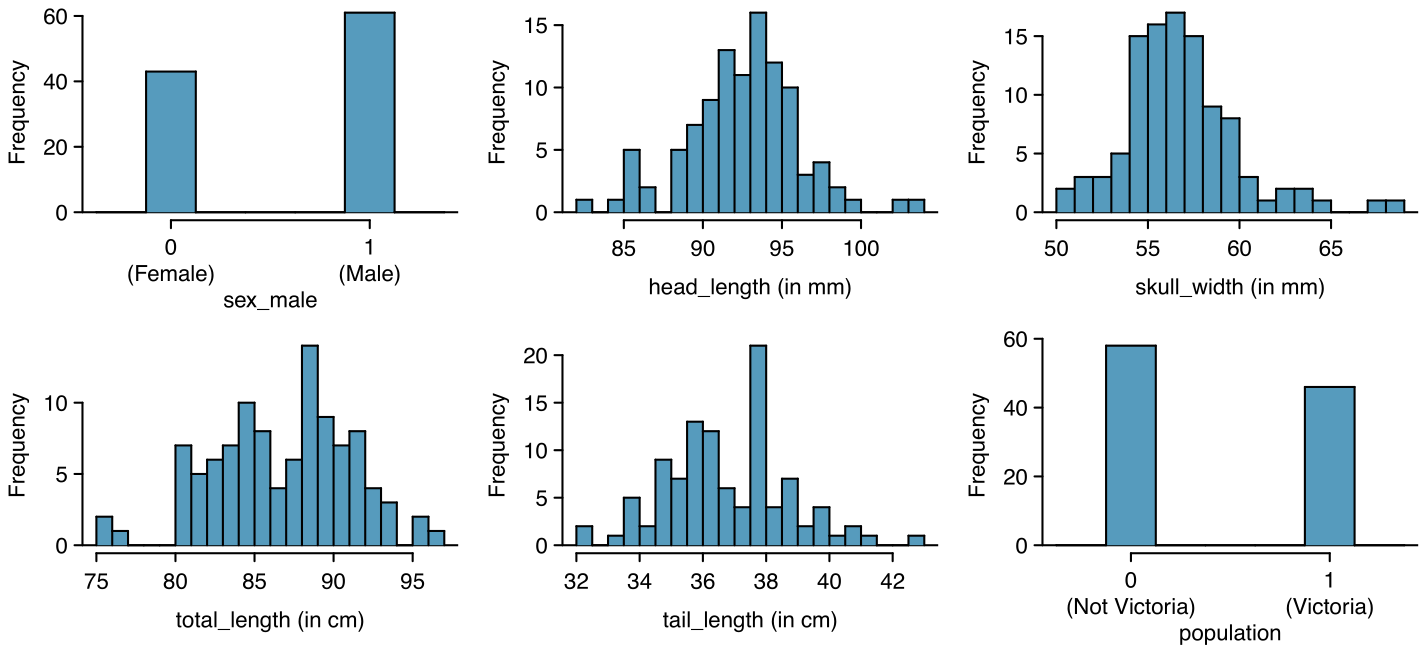
Possum classification, Part I. The common brushtail possum of the Australia region is a bit cuter than its distant cousin, the American opossum (see Figure 8.4). We consider 104 brushtail possums from two regions in Australia, where the possums may be considered a random sample from the population. The first region is Victoria, which is in the eastern half of Australia and traverses the southern coast. The second region consists of New South Wales and Queensland, which make up eastern and northeastern Australia. We use logistic regression to differentiate between possums in these two regions. The outcome variable, called population, takes value 1 when a possum is from Victoria and 0 when it is from New South Wales or Queensland. We consider five predictors: sex_ male (an indicator for a possum being male), head_ length, skull_ width, total_ length, and tail_ length. Each variable is summarized in a histogram. The full logistic regression model and a reduced model after variable selection are summarized in the table.

	Full Model				Reduced Model

	Estimate	SE	Z	Pr( $>$ $\|$ ⁠Z⁠ $\|$ ⁠)	Estimate	SE	Z	Pr( $>$ $\|$ ⁠Z⁠ $\|$ ⁠)

(Intercept)	39.2349	11.5368	3.40	0.0007	33.5095	9.9053	3.38	0.0007
sex_ male	-1.2376	0.6662	-1.86	0.0632	-1.4207	0.6457	-2.20	0.0278
head_ length	-0.1601	0.1386	-1.16	0.2480
skull_ width	-0.2012	0.1327	-1.52	0.1294	-0.2787	0.1226	-2.27	0.0231
total_ length	0.6488	0.1531	4.24	0.0000	0.5687	0.1322	4.30	0.0000
tail_ length	-1.8708	0.3741	-5.00	0.0000	-1.8057	0.3599	-5.02	0.0000

(a)

Examine each of the predictors. Are there any outliers that are likely to have a very large influence on the logistic regression model?

(b)

The summary table for the full model indicates that at least one variable should be eliminated when using the p-value approach for variable selection: head_ length. The second component of the table summarizes the reduced model following variable selection. Explain why the remaining estimates change between the two models.

Answer (2 parts)

(a)

There are a few potential outliers, e.g. on the left in the total_ length variable, but nothing that will be of serious concern in a data set this large.

(b)

When coefficient estimates are sensitive to which variables are included in the model, this typically indicates that some variables are collinear. For example, a possum’s gender may be related to its head length, which would explain why the coefficient (and p-value) for sex_ male changed when we removed the head_ length variable. Likewise, a possum’s skull width is likely to be related to its head length, probably even much more closely related than the head length was to gender.

9.17 §9.5 source ↗

Possum classification, Part II. A logistic regression model was proposed for classifying common brushtail possums into their two regions in Exercise 9.15. The outcome variable took value 1 if the possum was from Victoria and 0 otherwise.


	Estimate	SE	Z	Pr( $>$ $\|$ ⁠Z⁠ $\|$ ⁠)

(Intercept)	33.5095	9.9053	3.38	0.0007
sex_ male	-1.4207	0.6457	-2.20	0.0278
skull_ width	-0.2787	0.1226	-2.27	0.0231
total_ length	0.5687	0.1322	4.30	0.0000
tail_ length	-1.8057	0.3599	-5.02	0.0000

(a)

Write out the form of the model. Also identify which of the variables are positively associated when controlling for other variables.

(b)

Suppose we see a brushtail possum at a zoo in the US, and a sign says the possum had been captured in the wild in Australia, but it doesn’t say which part of Australia. However, the sign does indicate that the possum is male, its skull is about 63 mm wide, its tail is 37 cm long, and its total length is 83 cm. What is the reduced model’s computed probability that this possum is from Victoria? How confident are you in the model’s accuracy of this probability calculation?

Six plots are shown for the distributions of each predictor variable. For the ”sex_male” categorical variable, about 42 observations are ”0 (female)” and 65 are ”1 (male)”. For the ”head_length (in mm)” variable, a histogram is shown that is approximately bell-shaped, centered at about 93, and has a standard deviation of about 3. For the ”skull_width (in mm)” variable, a histogram is shown for a slightly right-skewed distribution is shown with its peak at about 56 and a standard deviation of about 3. For the ”total_length (in cm)” variable, a histogram is shown with most values ranging from about 80 to 95, with no major outliers. For the ”tail_length (in cm)” variable, a histogram is shown with most data between about 33 and 42, with no major outliers. For the ”population” categorical variable, about 58 observations are ”0 (Not Victoria)” and 45 are ”1 (Victoria)”. — Exercise 9.15 in the book ↗

Answer (2 parts)

(a)

The logistic model relating ${\hat{p}}_{i}$ to the predictors may be written as $\log (\frac{{\hat{p}}_{i}}{1 - {\hat{p}}_{i}}) =$ $33.5095 -$ $1.4207 \times s e x_m a l e_{i} -$ $0.2787 \times s k u l l_w i d t h_{i} +$ $0.5687 \times t o t a l_l e n g t h_{i} -$ $1.8057 \times t a i l_l e n g t h_{i}$ ⁠. Only total_ length has a positive association with a possum being from Victoria.

(b)

$\hat{p} = 0.0062$ ⁠. While the probability is very near zero, we have not run diagnostics on the model. We might also be a little skeptical that the model will remain accurate for a possum found in a US zoo. For example, perhaps the zoo selected a possum with specific characteristics but only looked in one region. On the other hand, it is encouraging that the possum was caught in the wild. (Answers regarding the reliability of the model probability will vary.)

9.19 §9.R source ↗

Multiple regression fact checking. Determine which of the following statements are true and false. For each statement that is false, explain why it is false.

(a)

If predictors are collinear, then removing one variable will have no influence on the point estimate of another variable’s coefficient.

(b)

Suppose a numerical variable $x$ has a coefficient of $b_{1} = 2.5$ in the multiple regression model. Suppose also that the first observation has $x_{1} = 7.2$ ⁠, the second observation has a value of $x_{1} = 8.2$ ⁠, and these two observations have the same values for all other predictors. Then the predicted value of the second observation will be 2.5 higher than the prediction of the first observation based on the multiple regression model.

(c)

If a regression model’s first variable has a coefficient of $b_{1} = 5.7$ ⁠, then if we are able to influence the data so that an observation will have its $x_{1}$ be 1 larger than it would otherwise, the value $y_{1}$ for this observation would increase by 5.7.

(d)

Suppose we fit a multiple regression model based on a data set of 472 observations. We also notice that the distribution of the residuals includes some skew but does not include any particularly extreme outliers. Because the residuals are not nearly normal, we should not use this model and require more advanced methods to model these data.

Answer (4 parts)

(a)

False. When predictors are collinear, it means they are correlated, and the inclusion of one variable can have a substantial influence on the point estimate (and standard error) of another.

(b)

True.

(c)

False. This would only be the case if the data was from an experiment and $x_{1}$ was one of the variables set by the researchers. (Multiple regression can be useful for forming hypotheses about causal relationships, but it offers zero guarantees.)

(d)

False. We should check normality like we would for inference for a single mean: we look for particularly extreme outliers if $n \geq 30$ or for clear outliers if $n < 30$ ⁠.

9.21 §9.R source ↗

Spam filtering, Part I. Spam filters are built on principles similar to those used in logistic regression. We fit a probability that each message is spam or not spam. We have several email variables for this problem: to_multiple, cc, attach, dollar, winner, inherit, password, format, re_subj, exclaim_subj, and sent_email. We won’t describe what each variable means here for the sake of brevity, but each is either a numerical or indicator variable.

(a)

For variable selection, we fit the full model, which includes all variables, and then we also fit each model where we’ve dropped exactly one of the variables. In each of these reduced models, the AIC value for the model is reported below. Based on these results, which variable, if any, should we drop as part of model selection? Explain.

Variable Dropped	AIC
None Dropped	1863.50
to_multiple	2023.50
cc	1863.18
attach	1871.89
dollar	1879.70
winner	1885.03
inherit	1865.55
password	1879.31
format	2008.85
re_subj	1904.60
exclaim_subj	1862.76
sent_email	1958.18

See the next page for part (b).

(b)

Consider the following model selection stage. Here again we’ve computed the AIC for each leave-one-variable-out model. Based on the results, which variable, if any, should we drop as part of model selection? Explain.

Variable Dropped	AIC
None Dropped	1862.41
to_multiple	2019.55
attach	1871.17
dollar	1877.73
winner	1884.95
inherit	1864.52
password	1878.19
format	2007.45
re_subj	1902.94
sent_email	1957.56

Answer (2 parts)

(a)

exclaim_subj should be removed, since it’s removal reduces AIC the most (and the resulting model has lower AIC than the None Dropped model).

(b)

Removing any variable will increase AIC, so we should not remove any variables from this set.

9.23 §9.R source ↗

Spam filtering, Part II. In Exercise 9.21, we encountered a data set where we applied logistic regression to aid in spam classification for individual emails. In this exercise, we’ve taken a small set of these variables and fit a formal model with the following output:

	Estimate	Std. Error	z value	Pr( $>$ $\|$ ⁠z⁠ $\|$ ⁠)
(Intercept)	-0.8124	0.0870	-9.34	0.0000
to_multiple	-2.6351	0.3036	-8.68	0.0000
winner	1.6272	0.3185	5.11	0.0000
format	-1.5881	0.1196	-13.28	0.0000
re_subj	-3.0467	0.3625	-8.40	0.0000

(a)

Write down the model using the coefficients from the model fit.

(b)

Suppose we have an observation where $𝚝𝚘_𝚖𝚞𝚕𝚝𝚒𝚙𝚕𝚎 = 0$ ⁠, $𝚠𝚒𝚗𝚗𝚎𝚛 = 1$ ⁠, $𝚏𝚘𝚛𝚖𝚊𝚝 = 0$ ⁠, and $𝚛𝚎_𝚜𝚞𝚋𝚓 = 0$ ⁠. What is the predicted probability that this message is spam?

(c)

Put yourself in the shoes of a data scientist working on a spam filter. For a given message, how high must the probability a message is spam be before you think it would be reasonable to put it in a spambox (which the user is unlikely to check)? What tradeoffs might you consider? Any ideas about how you might make your spam-filtering system even better from the perspective of someone using your email service?

Exercise 9.21 in the book ↗

(a) For variable selection, we fit the full model, which includes all variables, and then we also fit each model where we’ve dropped exactly one of the variables. In each of these reduced models, the AIC value for the model is reported below. Based on these results, which variable, if any, should we drop as part of model selection? Explain.

Variable Dropped	AIC
None Dropped	1863.50
to_multiple	2023.50
cc	1863.18
attach	1871.89
dollar	1879.70
winner	1885.03
inherit	1865.55
password	1879.31
format	2008.85
re_subj	1904.60
exclaim_subj	1862.76
sent_email	1958.18

See the next page for part (b).

(b) Consider the following model selection stage. Here again we’ve computed the AIC for each leave-one-variable-out model. Based on the results, which variable, if any, should we drop as part of model selection? Explain.

Variable Dropped	AIC
None Dropped	1862.41
to_multiple	2019.55
attach	1871.17
dollar	1877.73
winner	1884.95
inherit	1864.52
password	1878.19
format	2007.45
re_subj	1902.94
sent_email	1957.56

Answer. (a) exclaim_subj should be removed, since it’s removal reduces AIC the most (and the resulting model has lower AIC than the None Dropped model). (b) Removing any variable will increase AIC, so we should not remove any variables from this set.

Answer (3 parts)

(a)

The equation is:

$\begin{matrix} \log (\frac{p_{i}}{1 - p_{i}}) & = - 0.8124 \\ - 2.6351 \times to_multiple \\ + 1.6272 \times winner \\ - 1.5881 \times format \\ - 3.0467 \times re_subj \end{matrix}$

(b)

First find $\log (\frac{p}{1 - p})$ ⁠, then solve for $p$ ⁠:

$\begin{matrix} \log (\frac{p}{1 - p}) \\ = - 0.8124 - 2.6351 \times 0 + 1.6272 \times 1 \\ - 1.5881 \times 0 - 3.0467 \times 0 \\ = 0.8148 \\ \frac{p}{1 - p} = e^{0.8148} \to p = 0.693 \end{matrix}$

(c)

It should probably be pretty high, since it could be very disruptive to the person using the email service if they are missing emails that aren’t spam. Even only a 90% chance that a message is spam is probably enough to warrant keeping it in the inbox. Maybe a probability of 99% would be a reasonable cutoff. As for other ideas to make it even better, it may be worth building a second model that tries to classify the importance of an email message. If we have both the spam model and the importance model, we now have a better way to think about cost-benefit tradeoffs. For instance, perhaps we would be willing to have a lower probability-of-spam threshold for messages we were confident were not important, and perhaps we want an even higher probability threshold (e.g. 99.99%) for emails we are pretty sure are important.

End of the book.

Exercises and answers are adapted from OpenIntro Statistics by David Diez, Mine Çetinkaya-Rundel and Christopher D Barr, which is free to read and download, and are used under the CC BY-SA 3.0 licence. They are taken from the book’s LaTeX source and set for the web, so they may differ slightly from the printed page. This adaptation is released under the same licence and is neither affiliated with nor endorsed by Diez, Çetinkaya-Rundel and Barr or OpenIntro.