Every problem in the chapter beside the book’s answer, a chapter at a time as you scroll.
Chapter 7: Inference for numerical data
48 problems · 11 figuresGuided Practice 7.5 §7.1 source ↗
What proportion of the -distribution with 19 degrees of freedom falls above -1.79 units? Use your preferred method for finding tail areas.
Answer
We want to find the shaded area above -1.79 (we leave the picture to you). The lower tail area has an area of 0.0447, so the upper area would have an area of .
Guided Practice 7.10 §7.1 source ↗
The FDA’s webpage provides some data on mercury content of fish. Based on a sample of 15 croaker white fish (Pacific), a sample mean and standard deviation were computed as 0.287 and 0.069 ppm (parts per million), respectively. The 15 observations ranged from 0.18 to 0.41 ppm. We will assume these observations are independent. Based on the summary statistics of the data, do you have any objections to the normality condition of the individual observations?
Answer
The sample size is under 30, so we check for obvious outliers: since all observations are within 2 standard deviations of the mean, there are no such clear outliers.
Guided Practice 7.12 §7.1 source ↗
Using the information and results of Guided Practice 7.10 and Example 7.11, compute a 90% confidence interval for the average mercury content of croaker white fish (Pacific).
The FDA’s webpage provides some data on mercury content of fish. Based on a sample of 15 croaker white fish (Pacific), a sample mean and standard deviation were computed as 0.287 and 0.069 ppm (parts per million), respectively. The 15 observations ranged from 0.18 to 0.41 ppm. We will assume these observations are independent. Based on the summary statistics of the data, do you have any objections to the normality condition of the individual observations?
Answer. The sample size is under 30, so we check for obvious outliers: since all observations are within 2 standard deviations of the mean, there are no such clear outliers.
Estimate the standard error of ppm using the data summaries in Guided Practice 7.10. If we are to use the -distribution to create a 90% confidence interval for the actual mean of the mercury content, identify the degrees of freedom and .
Answer. The standard error: .
Degrees of freedom: .
Since the goal is a 90% confidence interval, we choose so that the two-tail area is 0.1: .
Answer
. We are 90% confident that the average mercury content of croaker white fish (Pacific) is between 0.256 and 0.318 ppm.
Guided Practice 7.13 §7.1 source ↗
The 90% confidence interval from Guided Practice 7.12 is 0.256 ppm to 0.318 ppm. Can we say that 90% of croaker white fish (Pacific) have mercury levels between 0.256 and 0.318 ppm?
Using the information and results of Guided Practice 7.10 and Example 7.11, compute a 90% confidence interval for the average mercury content of croaker white fish (Pacific).
Answer. . We are 90% confident that the average mercury content of croaker white fish (Pacific) is between 0.256 and 0.318 ppm.
Answer
No, a confidence interval only provides a range of plausible values for a population parameter, in this case the population mean. It does not describe what we might observe for individual observations.
Guided Practice 7.14 §7.1 source ↗
What are appropriate hypotheses for this context?
Answer
: The average 10-mile run time was the same for 2006 and 2017. minutes. : The average 10-mile run time for 2017 was different than that of 2006. minutes.
Guided Practice 7.15 §7.1 source ↗
The data come from a simple random sample of all participants, so the observations are independent. However, should we be worried about the normality condition? See Figure 7.7 for a histogram of the differences and evaluate if we can move forward.
time for the sample Cherry Blossom Race data.Answer
With a sample of 100, we should only be concerned if there is are particularly extreme outliers. The histogram of the data doesn’t show any outliers of concern (and arguably, no outliers at all).
7.1 §7.1 source ↗
Identify the critical . An independent random sample is selected from an approximately normal population with unknown standard deviation. Find the degrees of freedom and the critical -value (t) for the given sample size and confidence level.
, CL = 90%
, CL = 98%
, CL = 95%
, CL = 99%
Answer (4 parts)
, (column with two tails of 0.10, row with ).
, (column with two tails of 0.02, row with ).
, .
, .
7.3 §7.1 source ↗
Find the p-value, Part I. An independent random sample is selected from an approximately normal population with an unknown standard deviation. Find the p-value for the given sample size and test statistic. Also determine if the null hypothesis would be rejected at .
,
,
,
,
Answer (4 parts)
0.085, do not reject .
0.003, reject .
0.438, do not reject .
0.042, reject .
7.5 §7.1 source ↗
Working backwards, Part I. A 95% confidence interval for a population mean, , is given as (18.985, 21.015). This confidence interval is based on a simple random sample of 36 observations. Calculate the sample mean and standard deviation. Assume that all conditions necessary for inference are satisfied. Use the -distribution in any calculations.
Answer
The mean is the midpoint: . Identify the margin of error: , then use and in the formula for margin of error to identify .
7.7 §7.1 source ↗
Sleep habits of New Yorkers. New York is known as “the city that never sleeps". A random sample of 25 New Yorkers were asked how much sleep they get per night. Statistical summaries of these data are shown below. The point estimate suggests New Yorkers sleep less than 8 hours a night on average. Is the result statistically significant?
| n | s | min | max | |
| 25 | 7.73 | 0.77 | 6.17 | 9.78 |
Write the hypotheses in symbols and in words.
Check conditions, then calculate the test statistic, , and the associated degrees of freedom.
Find and interpret the p-value in this context. Drawing a picture may be helpful.
What is the conclusion of the hypothesis test?
If you were to construct a 90% confidence interval that corresponded to this hypothesis test, would you expect 8 hours to be in the interval?
Answer (5 parts)
: (New Yorkers sleep 8 hrs per night on average.) : (New Yorkers sleep less or more than 8 hrs per night on average.)
Independence: The sample is random. The min/max suggest there are no concerning outliers. . .
p-value . If in fact the true population mean of the amount New Yorkers sleep per night was 8 hours, the probability of getting a random sample of 25 New Yorkers where the average amount of sleep is 7.73 hours per night or less (or 8.27 hours or more) is 0.093.
Since p-value 0.05, do not reject . The data do not provide strong evidence that New Yorkers sleep more or less than 8 hours per night on average.
No, since the p-value is smaller than .
7.9 §7.1 source ↗
Find the mean. You are given the following hypotheses:
We know that the sample standard deviation is 8 and the sample size is 20. For what sample mean would the p-value be equal to 0.05? Assume that all conditions necessary for inference are satisfied.
Answer
is either -2.09 or 2.09. Then is one of the following:
7.11 §7.1 source ↗
Play the piano. Georgianna claims that in a small city renowned for its music school, the average child takes less than 5 years of piano lessons. We have a random sample of 20 children from the city, with a mean of 4.6 years of piano lessons and a standard deviation of 2.2 years.
Evaluate Georgianna’s claim (or that the opposite might be true) using a hypothesis test.
Construct a 95% confidence interval for the number of years students in this city take piano lessons, and interpret it in context of the data.
Do your results from the hypothesis test and the confidence interval agree? Explain your reasoning.
Answer (3 parts)
We will conduct a 1-sample -test. : . : . We’ll use . This is a random sample, so the observations are independent. To proceed, we assume the distribution of years of piano lessons is approximately normal. . The test statistic is . . The one-tail area is about 0.21, so the p-value is about 0.42, which is bigger than and we do not reject . That is, we do not have sufficiently strong evidence to reject the notion that the average is 5 years.
Using and , the confidence interval is (3.57, 5.63). We are 95% confident that the average number of years a child takes piano lessons in this city is 3.57 to 5.63 years.
They agree, since we did not reject the null hypothesis and the null value of 5 was in the -interval.
7.13 §7.1 source ↗
Car insurance savings. A market researcher wants to evaluate car insurance savings at a competing company. Based on past studies he is assuming that the standard deviation of savings is $100. He wants to collect data such that he can get a margin of error of no more than $10 at a 95% confidence level. How large of a sample should he collect?
Answer
If the sample is large, then the margin of error will be about . We want this value to be less than 10, which leads to , meaning we need a sample size of at least 385 (round up for sample size calculations!).
Guided Practice 7.19 §7.2 source ↗
Create a 95% confidence interval for the average price difference between books at the UCLA bookstore and books on Amazon.
Answer
Conditions have already verified and the standard error computed in Example 7.17. To find the interval, identify using statistical software or the -table (), and plug it, the point estimate, and the standard error into the confidence interval formula:
We are 95% confident that Amazon is, on average, between $0.32 and $6.84 less expensive than the UCLA Bookstore for UCLA course books.
Set up a hypothesis test to determine whether, on average, there is a difference between Amazon’s price for a book and the UCLA bookstore’s price. Also, check the conditions for whether we can move forward with the test using the -distribution.
Answer. We are considering two scenarios: there is no difference or there is some difference in average prices.
: . There is no difference in the average textbook price.
: . There is a difference in average prices.
Next, we check the independence and normality conditions. The observations are based on a simple random sample, so independence is reasonable. While there are some outliers, and none of the outliers are particularly extreme, so the normality of is satisfied. With these conditions satisfied, we can move forward with the -distribution.
Guided Practice 7.20 §7.2 source ↗
We have strong evidence that Amazon is, on average, less expensive. How should this conclusion affect UCLA student buying habits? Should UCLA students always buy their books on Amazon?
Answer
The average price difference is only mildly useful for this question. Examine the distribution shown in Figure 7.9. There are certainly a handful of cases where Amazon prices are far below the UCLA Bookstore’s, which suggests it is worth checking Amazon (and probably other online sites) before purchasing. However, in many cases the Amazon price is above what the UCLA Bookstore charges, and most of the time the price isn’t that different. Ultimately, if getting a book immediately from the bookstore is notably more convenient, e.g. to get started on reading or homework, it’s likely a good idea to go with the UCLA Bookstore unless the price difference on a specific book happens to be quite large.
For reference, this is a very different result from what we (the authors) had seen in a similar data set from 2010. At that time, Amazon prices were almost uniformly lower than those of the UCLA Bookstore’s and by a large margin, making the case to use Amazon over the UCLA Bookstore quite compelling at that time. Now we frequently check multiple websites to find the best price.
7.15 §7.2 source ↗
Air quality. Air quality measurements were collected in a random sample of 25 country capitals in 2013, and then again in the same cities in 2014. We would like to use these data to compare average air quality between the two years. Should we use a paired or non-paired test? Explain your reasoning.
Answer
Paired, data are recorded in the same cities at two different time points. The air quality in a city at one point is not independent of the air quality in the same city at another time point.
7.17 §7.2 source ↗
Paired or not? Part I. In each of the following scenarios, determine if the data are paired.
Compare pre- (beginning of semester) and post-test (end of semester) scores of students.
Assess gender-related salary gap by comparing salaries of randomly sampled men and women.
Compare artery thicknesses at the beginning of a study and after 2 years of taking Vitamin E for the same group of patients.
Assess effectiveness of a diet regimen by comparing the before and after weights of subjects.
Answer (4 parts)
Since it’s the same students at the beginning and the end of the semester, there is a pairing between the datasets, for a given student their beginning and end of semester grades are dependent.
Since the subjects were sampled randomly, each observation in the men’s group does not have a special correspondence with exactly one observation in the other (women’s) group.
Since it’s the same subjects at the beginning and the end of the study, there is a pairing between the datasets, for a subject student their beginning and end of semester artery thickness are dependent.
Since it’s the same subjects at the beginning and the end of the study, there is a pairing between the datasets, for a subject student their beginning and end of semester weights are dependent.
7.19 §7.2 source ↗
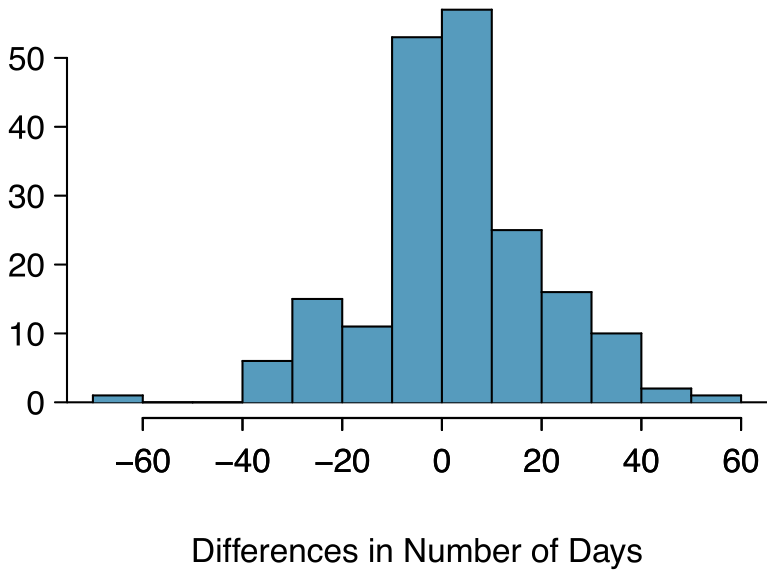
Global warming, Part I. Let’s consider a limited set of climate data, examining temperature differences in 1948 vs 2018. We sampled 197 locations from the National Oceanic and Atmospheric Administration’s (NOAA) historical data, where the data was available for both years of interest. We want to know: were there more days with temperatures exceeding 90°F in 2018 or in 1948? The difference in number of days exceeding 90°F (number of days in 2018 - number of days in 1948) was calculated for each of the 197 locations. The average of these differences was 2.9 days with a standard deviation of 17.2 days. We are interested in determining whether these data provide strong evidence that there were more days in 2018 that exceeded 90°F from NOAA’s weather stations.
(a) Is there a relationship between the observations collected in 1948 and 2018? Or are the observations in the two groups independent? Explain.
(b) Write hypotheses for this research in symbols and in words.
(c) Check the conditions required to complete this test. A histogram of the differences is given to the right.
(d) Calculate the test statistic and find the p-value.
(e) Use to evaluate the test, and interpret your conclusion in context.
(f) What type of error might we have made? Explain in context what the error means.
(g) Based on the results of this hypothesis test, would you expect a confidence interval for the average difference between the number of days exceeding 90°F from 1948 and 2018 to include 0? Explain your reasoning.
Answer (7 parts)
For each observation in one data set, there is exactly one specially corresponding observation in the other data set for the same geographic location. The data are paired.
(There is no difference in average number of days exceeding 90°F in 1948 and 2018 for NOAA stations.) (There is a difference.)
Locations were randomly sampled, so independence is reasonable. The sample size is at least 30, so we’re just looking for particularly extreme outliers: none are present (the observation off left in the histogram would be considered a clear outlier, but not a particularly extreme one). Therefore, the conditions are satisfied.
. with degrees of freedom . This leads to a one-tail area of 0.0096 and a p-value of about 0.019.
Since the p-value is less than 0.05, we reject . The data provide strong evidence that NOAA stations observed more 90°F days in 2018 than in 1948.
Type 1 Error, since we may have incorrectly rejected . This error would mean that NOAA stations did not actually observe a decrease, but the sample we took just so happened to make it appear that this was the case.
No, since we rejected , which had a null value of 0.
7.21 §7.2 source ↗
Global warming, Part II. We considered the change in the number of days exceeding 90°F from 1948 and 2018 at 197 randomly sampled locations from the NOAA database in Exercise 7.19. The mean and standard deviation of the reported differences are 2.9 days and 17.2 days.
Calculate a 90% confidence interval for the average difference between number of days exceeding 90°F between 1948 and 2018. We’ve already checked the conditions for you.
Interpret the interval in context.
Does the confidence interval provide convincing evidence that there were more days exceeding 90°F in 2018 than in 1948 at NOAA stations? Explain.
Global warming, Part I. Let’s consider a limited set of climate data, examining temperature differences in 1948 vs 2018. We sampled 197 locations from the National Oceanic and Atmospheric Administration’s (NOAA) historical data, where the data was available for both years of interest. We want to know: were there more days with temperatures exceeding 90°F in 2018 or in 1948? The difference in number of days exceeding 90°F (number of days in 2018 - number of days in 1948) was calculated for each of the 197 locations. The average of these differences was 2.9 days with a standard deviation of 17.2 days. We are interested in determining whether these data provide strong evidence that there were more days in 2018 that exceeded 90°F from NOAA’s weather stations.
(a) Is there a relationship between the observations collected in 1948 and 2018? Or are the observations in the two groups independent? Explain.
(b) Write hypotheses for this research in symbols and in words.
(c) Check the conditions required to complete this test. A histogram of the differences is given to the right.
(d) Calculate the test statistic and find the p-value.
(e) Use to evaluate the test, and interpret your conclusion in context.
(f) What type of error might we have made? Explain in context what the error means.
(g) Based on the results of this hypothesis test, would you expect a confidence interval for the average difference between the number of days exceeding 90°F from 1948 and 2018 to include 0? Explain your reasoning.
Answer. (a) For each observation in one data set, there is exactly one specially corresponding observation in the other data set for the same geographic location. The data are paired. (b) (There is no difference in average number of days exceeding 90°F in 1948 and 2018 for NOAA stations.) (There is a difference.) (c) Locations were randomly sampled, so independence is reasonable. The sample size is at least 30, so we’re just looking for particularly extreme outliers: none are present (the observation off left in the histogram would be considered a clear outlier, but not a particularly extreme one). Therefore, the conditions are satisfied. (d) . with degrees of freedom . This leads to a one-tail area of 0.0096 and a p-value of about 0.019. (e) Since the p-value is less than 0.05, we reject . The data provide strong evidence that NOAA stations observed more 90°F days in 2018 than in 1948. (f) Type 1 Error, since we may have incorrectly rejected . This error would mean that NOAA stations did not actually observe a decrease, but the sample we took just so happened to make it appear that this was the case. (g) No, since we rejected , which had a null value of 0.
Answer (3 parts)
and . .
We are 90% confident that there was an increase of 0.87 to 4.93 in the average number of days that hit 90°F in 2018 relative to 1948 for NOAA stations.
Yes, since the interval lies entirely above 0.
Guided Practice 7.24 §7.3 source ↗
The summary statistics in Figure 7.15 may be useful for this Guided Practice.
1. What is the point estimate of the population difference, ?
2. Compute the standard error of the point estimate from part (a).
| smoker | nonsmoker | |
| mean | 6.78 | 7.18 |
| st. dev. | 1.43 | 1.60 |
| samp. size | 50 | 100 |
ncbirths data set.Answer (2 parts)
The difference in sample means is an appropriate point estimate: .
The standard error of the estimate can be calculated using the standard error formula:
Guided Practice 7.26 §7.3 source ↗
We’ve seen much research suggesting smoking is harmful during pregnancy, so how could we fail to reject the null hypothesis in Example 7.25?
Complete the hypothesis test started in Example 7.23 and Guided Practice 7.24. Use a significance level of . For reference, , , and the sample sizes were and .
Answer. We can find the test statistic for this test using the values from Guided Practice 7.24:
The p-value is represented by the two shaded tails in the following plot:
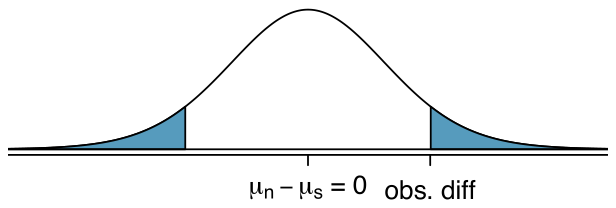
We find the single tail area using software (or the -table in Appendix C.2). We’ll use the smaller of and as the degrees of freedom: . The one tail area is 0.065; doubling this value gives the two-tail area and p-value, 0.135.
The p-value is larger than the significance value, 0.05, so we do not reject the null hypothesis. There is insufficient evidence to say there is a difference in average birth weight of newborns from North Carolina mothers who did smoke during pregnancy and newborns from North Carolina mothers who did not smoke during pregnancy.
Answer
It is possible that there is a difference but we did not detect it. If there is a difference, we made a Type 2 Error.
Guided Practice 7.27 §7.3 source ↗
If we made a Type 2 Error and there is a difference, what could we have done differently in data collection to be more likely to detect the difference?
Answer
We could have collected more data. If the sample sizes are larger, we tend to have a better shot at finding a difference if one exists. In fact, this is exactly what we would find if we examined a larger data set!
Guided Practice 7.28 §7.3 source ↗
Construct hypotheses to evaluate whether the observed difference in sample means, , is due to chance. We will later evaluate these hypotheses using .
Answer
: the exams are equally difficult, on average. . : one exam was more difficult than the other, on average. .
Guided Practice 7.29 §7.3 source ↗
To evaluate the hypotheses in Guided Practice 7.28 using the -distribution, we must first verify conditions.
1. Does it seem reasonable that the scores are independent?
2. Any concerns about outliers?
Construct hypotheses to evaluate whether the observed difference in sample means, , is due to chance. We will later evaluate these hypotheses using .
Answer. : the exams are equally difficult, on average. . : one exam was more difficult than the other, on average. .
Answer (2 parts)
Since the exams were shuffled, the “treatment” in this case was randomly assigned, so independence within and between groups is satisfied.
The summary statistics suggest the data are roughly symmetric about the mean, and the min/max values don’t suggest any outliers of concern.
7.23 §7.3 source ↗
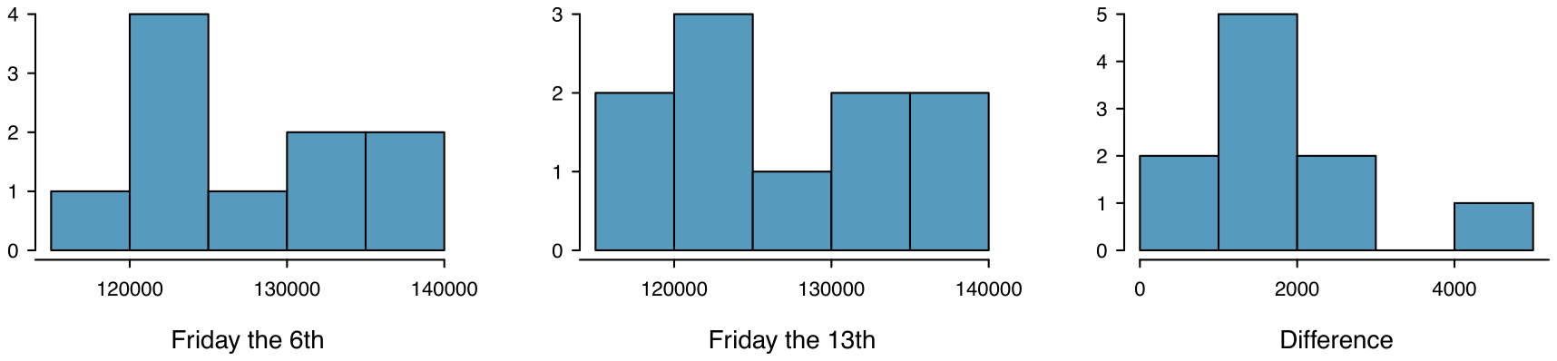
Friday the 13, Part I. In the early 1990’s, researchers in the UK collected data on traffic flow, number of shoppers, and traffic accident related emergency room admissions on Friday the 13 and the previous Friday, Friday the 6. The histograms below show the distribution of number of cars passing by a specific intersection on Friday the 6 and Friday the 13 for many such date pairs. Also given are some sample statistics, where the difference is the number of cars on the 6th minus the number of cars on the 13th.
| 6 | 13 | Diff. | |
| 128,385 | 126,550 | 1,835 | |
| 7,259 | 7,664 | 1,176 | |
| 10 | 10 | 10 |
Are there any underlying structures in these data that should be considered in an analysis? Explain.
What are the hypotheses for evaluating whether the number of people out on Friday the 6 is different than the number out on Friday the 13?
Check conditions to carry out the hypothesis test from part (b).
Calculate the test statistic and the p-value.
What is the conclusion of the hypothesis test?
Interpret the p-value in this context.
What type of error might have been made in the conclusion of your test? Explain.
Answer (7 parts)
These data are paired. For example, the Friday the 13th in say, September 1991, would probably be more similar to the Friday the 6th in September 1991 than to Friday the 6th in another month or year.
Let . . .
Independence: The months selected are not random. However, if we think these dates are roughly equivalent to a simple random sample of all such Friday 6th/13th date pairs, then independence is reasonable. To proceed, we must make this strong assumption, though we should note this assumption in any reported results. Normality: With fewer than 10 observations, we would need to see clear outliers to be concerned. There is a borderline outlier on the right of the histogram of the differences, so we would want to report this in formal analysis results.
for p-value = 0.001.
Since p-value 0.05, reject . The data provide strong evidence that the average number of cars at the intersection is higher on Friday the 6 than on Friday the 13. (We should exercise caution about generalizing the interpretation to all intersections or roads.)
If the average number of cars passing the intersection actually was the same on Friday the 6 and , then the probability that we would observe a test statistic so far from zero is less than 0.01.
We might have made a Type 1 Error, i.e. incorrectly rejected the null hypothesis.
7.25 §7.3 source ↗
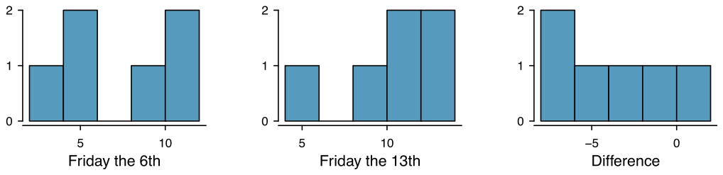
Friday the 13, Part II. The Friday the study reported in Exercise 7.23 also provides data on traffic accident related emergency room admissions. The distributions of these counts from Friday the 6 and Friday the 13 are shown below for six such paired dates along with summary statistics. You may assume that conditions for inference are met.
| 6 | 13 | diff | |
| Mean | 7.5 | 10.83 | -3.33 |
| SD | 3.33 | 3.6 | 3.01 |
| n | 6 | 6 | 6 |
Conduct a hypothesis test to evaluate if there is a difference between the average numbers of traffic accident related emergency room admissions between Friday the 6 and Friday the 13.
Calculate a 95% confidence interval for the difference between the average numbers of traffic accident related emergency room admissions between Friday the 6 and Friday the 13.
The conclusion of the original study states, “Friday 13th is unlucky for some. The risk of hospital admission as a result of a transport accident may be increased by as much as 52%. Staying at home is recommended.” Do you agree with this statement? Explain your reasoning.
Friday the 13, Part I. In the early 1990’s, researchers in the UK collected data on traffic flow, number of shoppers, and traffic accident related emergency room admissions on Friday the 13 and the previous Friday, Friday the 6. The histograms below show the distribution of number of cars passing by a specific intersection on Friday the 6 and Friday the 13 for many such date pairs. Also given are some sample statistics, where the difference is the number of cars on the 6th minus the number of cars on the 13th.
| 6 | 13 | Diff. | |
| 128,385 | 126,550 | 1,835 | |
| 7,259 | 7,664 | 1,176 | |
| 10 | 10 | 10 |
(a) Are there any underlying structures in these data that should be considered in an analysis? Explain.
(b) What are the hypotheses for evaluating whether the number of people out on Friday the 6 is different than the number out on Friday the 13?
(c) Check conditions to carry out the hypothesis test from part (b).
(d) Calculate the test statistic and the p-value.
(e) What is the conclusion of the hypothesis test?
(f) Interpret the p-value in this context.
(g) What type of error might have been made in the conclusion of your test? Explain.
Answer. (a) These data are paired. For example, the Friday the 13th in say, September 1991, would probably be more similar to the Friday the 6th in September 1991 than to Friday the 6th in another month or year.
(b) Let . . .
(c) Independence: The months selected are not random. However, if we think these dates are roughly equivalent to a simple random sample of all such Friday 6th/13th date pairs, then independence is reasonable. To proceed, we must make this strong assumption, though we should note this assumption in any reported results. Normality: With fewer than 10 observations, we would need to see clear outliers to be concerned. There is a borderline outlier on the right of the histogram of the differences, so we would want to report this in formal analysis results.
(d) for p-value = 0.001.
(e) Since p-value 0.05, reject . The data provide strong evidence that the average number of cars at the intersection is higher on Friday the 6 than on Friday the 13. (We should exercise caution about generalizing the interpretation to all intersections or roads.)
(f) If the average number of cars passing the intersection actually was the same on Friday the 6 and , then the probability that we would observe a test statistic so far from zero is less than 0.01.
(g) We might have made a Type 1 Error, i.e. incorrectly rejected the null hypothesis.
Answer (3 parts)
. . . . p-value . Since p-value 0.05, reject . The data provide strong evidence that the average number of traffic accident related emergency room admissions are different between Friday the 6 and Friday the 13. Furthermore, the data indicate that the direction of that difference is that accidents are lower on Friday the relative to Friday the 13.
(-6.49, -0.17).
This is an observational study, not an experiment, so we cannot so easily infer a causal intervention implied by this statement. It is true that there is a difference. However, for example, this does not mean that a responsible adult going out on Friday the has a higher chance of harm than on any other night.
7.27 §7.3 source ↗
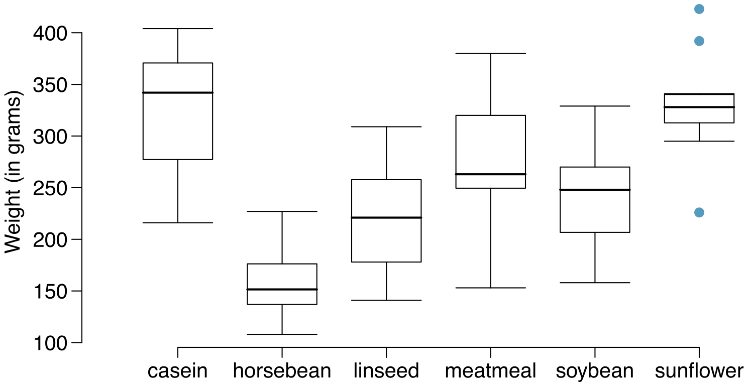
Chicken diet and weight, Part I. Chicken farming is a multi-billion dollar industry, and any methods that increase the growth rate of young chicks can reduce consumer costs while increasing company profits, possibly by millions of dollars. An experiment was conducted to measure and compare the effectiveness of various feed supplements on the growth rate of chickens. Newly hatched chicks were randomly allocated into six groups, and each group was given a different feed supplement. Below are some summary statistics from this data set along with box plots showing the distribution of weights by feed type.
| Mean | SD | n | |
| casein | 323.58 | 64.43 | 12 |
| horsebean | 160.20 | 38.63 | 10 |
| linseed | 218.75 | 52.24 | 12 |
| meatmeal | 276.91 | 64.90 | 11 |
| soybean | 246.43 | 54.13 | 14 |
| sunflower | 328.92 | 48.84 | 12 |
Describe the distributions of weights of chickens that were fed linseed and horsebean.
Do these data provide strong evidence that the average weights of chickens that were fed linseed and horsebean are different? Use a 5% significance level.
What type of error might we have committed? Explain.
Would your conclusion change if we used ?
Answer (4 parts)
Chicken fed linseed weighed an average of 218.75 grams while those fed horsebean weighed an average of 160.20 grams. Both distributions are relatively symmetric with no apparent outliers. There is more variability in the weights of chicken fed linseed.
. .
We leave the conditions to you to consider.
, p-value . Since p-value 0.05, reject . The data provide strong evidence that there is a significant difference between the average weights of chickens that were fed linseed and horsebean.
Type 1 Error, since we rejected .
Yes, since p-value 0.01, we would not have rejected .
7.29 §7.3 source ↗
Chicken diet and weight, Part II. Casein is a common weight gain supplement for humans. Does it have an effect on chickens? Using data provided in Exercise 7.27, test the hypothesis that the average weight of chickens that were fed casein is different than the average weight of chickens that were fed soybean. If your hypothesis test yields a statistically significant result, discuss whether or not the higher average weight of chickens can be attributed to the casein diet. Assume that conditions for inference are satisfied.
Chicken diet and weight, Part I. Chicken farming is a multi-billion dollar industry, and any methods that increase the growth rate of young chicks can reduce consumer costs while increasing company profits, possibly by millions of dollars. An experiment was conducted to measure and compare the effectiveness of various feed supplements on the growth rate of chickens. Newly hatched chicks were randomly allocated into six groups, and each group was given a different feed supplement. Below are some summary statistics from this data set along with box plots showing the distribution of weights by feed type.
| Mean | SD | n | |
| casein | 323.58 | 64.43 | 12 |
| horsebean | 160.20 | 38.63 | 10 |
| linseed | 218.75 | 52.24 | 12 |
| meatmeal | 276.91 | 64.90 | 11 |
| soybean | 246.43 | 54.13 | 14 |
| sunflower | 328.92 | 48.84 | 12 |
(a) Describe the distributions of weights of chickens that were fed linseed and horsebean.
(b) Do these data provide strong evidence that the average weights of chickens that were fed linseed and horsebean are different? Use a 5% significance level.
(c) What type of error might we have committed? Explain.
(d) Would your conclusion change if we used ?
Answer. (a) Chicken fed linseed weighed an average of 218.75 grams while those fed horsebean weighed an average of 160.20 grams. Both distributions are relatively symmetric with no apparent outliers. There is more variability in the weights of chicken fed linseed.
(b) . .
We leave the conditions to you to consider.
, p-value . Since p-value 0.05, reject . The data provide strong evidence that there is a significant difference between the average weights of chickens that were fed linseed and horsebean.
(c) Type 1 Error, since we rejected .
(d) Yes, since p-value 0.01, we would not have rejected .
Answer
. . , p-value . Since p-value , reject . The data provide strong evidence that the average weight of chickens that were fed casein is different than the average weight of chickens that were fed soybean (with weights from casein being higher). Since this is a randomized experiment, the observed difference can be attributed to the diet.
7.31 §7.3 source ↗
Prison isolation experiment, Part I. Subjects from Central Prison in Raleigh, NC, volunteered for an experiment involving an “isolation” experience. The goal of the experiment was to find a treatment that reduces subjects’ psychopathic deviant T scores. This score measures a person’s need for control or their rebellion against control, and it is part of a commonly used mental health test called the Minnesota Multiphasic Personality Inventory (MMPI) test. The experiment had three treatment groups:
1. Four hours of sensory restriction plus a 15 minute “therapeutic" tape advising that professional help is available.
2. Four hours of sensory restriction plus a 15 minute “emotionally neutral” tape on training hunting dogs.
3. Four hours of sensory restriction but no taped message.
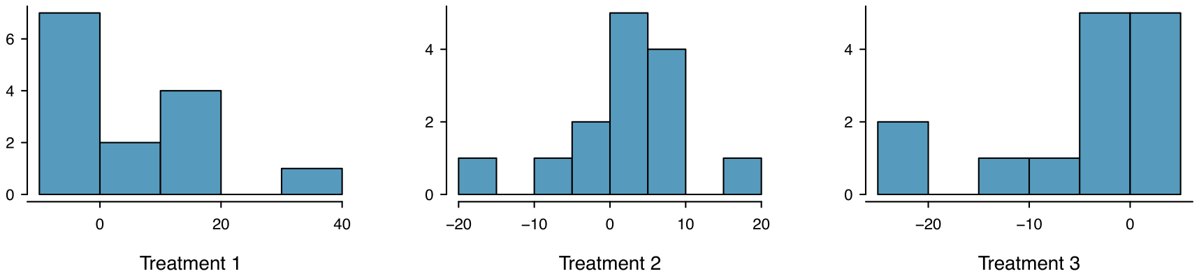
Forty-two subjects were randomly assigned to these treatment groups, and an MMPI test was administered before and after the treatment. Distributions of the differences between pre and post treatment scores (pre - post) are shown below, along with some sample statistics. Use this information to independently test the effectiveness of each treatment. Make sure to clearly state your hypotheses, check conditions, and interpret results in the context of the data.
| Tr 1 | Tr 2 | Tr 3 | |
| Mean | 6.21 | 2.86 | -3.21 |
| SD | 12.3 | 7.94 | 8.57 |
| n | 14 | 14 | 14 |
Answer
Let . : Treatment has no effect. : Treatment has an effect on P.D.T. scores, either positive or negative. Conditions: The subjects are randomly assigned to treatments, so independence within and between groups is satisfied. All three sample sizes are smaller than 30, so we look for clear outliers. There is a borderline outlier in the first treatment group. Since it is borderline, we will proceed, but we should report this caveat with any results. For all three groups: . p-value = 0.081, p-value = 0.200), (p-value = 0.185). We do not reject the null hypothesis for any of these groups. As earlier noted, there is some uncertainty about if the method applied is reasonable for the first group.
Guided Practice 7.36 §7.4 source ↗
Calculate the power to detect a change of -3 mmHg when using a sample size of 500 per group.
1. Determine the standard error (recall that the standard deviation for patients was expected to be about 12 mmHg).
2. Identify the null distribution and rejection regions.
3. Identify the alternative distribution when .
4. Compute the probability we reject the null hypothesis.
Answer (4 parts)
The standard error is given as .
&
The null distribution, rejection boundaries, and alternative distribution are shown below:
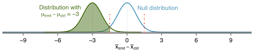
The rejection regions are the areas on the outside of the two dotted lines and are at .
The area of the alternative distribution where has been shaded. We compute the Z-score and find the tail area: . With 500 patients per group, we would be about 97.7% sure (or more) that we’d detect any effects that are at least 3 mmHg in size.
Guided Practice 7.38 §7.4 source ↗
Suppose the targeted power was 90% and we were using . How many standard errors should separate the centers of the null and alternative distribution, where the alternative distribution is centered at the minimum effect size of interest?
Answer
First, find the Z-score such that 90% of the distribution is below it: . Next, find the cutoffs for the rejection regions: . Then the difference in centers should be about .
Guided Practice 7.39 §7.4 source ↗
What are some considerations that are important in determining what the power should be for an experiment?
Answer
Answers will vary, but here are a few important considerations:
• Whether there is any risk to patients in the study.
• The cost of enrolling more patients.
• The potential downside of not detecting an effect of interest.
7.33 §7.4 source ↗
Increasing corn yield. A large farm wants to try out a new type of fertilizer to evaluate whether it will improve the farm’s corn production. The land is broken into plots that produce an average of 1,215 pounds of corn with a standard deviation of 94 pounds per plot. The owner is interested in detecting any average difference of at least 40 pounds per plot. How many plots of land would be needed for the experiment if the desired power level is 90%? Use . Assume each plot of land gets treated with either the current fertilizer or the new fertilizer.
Answer
Difference we care about: 40. Single tail of 90%: . Rejection region bounds: (if 5% significance level). Setting , subbing in , and solving for the sample size gives 116 plots of land for each fertilizer.
Guided Practice 7.42 §7.5 source ↗
The null hypothesis under consideration is the following: . Write the null and corresponding alternative hypotheses in plain language.
Answer
: The average on-base percentage is equal across the three positions. : The average on-base percentage varies across some (or all) groups.
Guided Practice 7.45 §7.5 source ↗
For the baseball data, and . Identify the degrees of freedom associated with MSG and MSE and verify the statistic is approximately 5.077.
Answer
There are groups, so . There are total observations, so . Then the statistic is computed as the ratio of and : . ( was computed by using values for and that were not rounded.)
Guided Practice 7.48 §7.5 source ↗
ANOVA was conducted for the midterm data, and summary results are shown in Figure 7.29. What should we conclude?
| Df | Sum Sq | Mean Sq | F value | Pr(F) | |
| lecture | 2 | 1290.11 | 645.06 | 3.48 | 0.0330 |
| Residuals | 161 | 29810.13 | 185.16 | ||
| on | |||||
Answer
The p-value of the test is 0.0330, less than the default significance level of 0.05. Therefore, we reject the null hypothesis and conclude that the difference in the average midterm scores are not due to chance.
7.35 §7.5 source ↗
Fill in the blank. When doing an ANOVA, you observe large differences in means between groups. Within the ANOVA framework, this would most likely be interpreted as evidence strongly favoring the hypothesis.
Answer
Alternative.
7.37 §7.5 source ↗
Chicken diet and weight, Part III. In Exercises 7.27 and 7.29 we compared the effects of two types of feed at a time. A better analysis would first consider all feed types at once: casein, horsebean, linseed, meat meal, soybean, and sunflower. The ANOVA output below can be used to test for differences between the average weights of chicks on different diets.
| Df | Sum Sq | Mean Sq | F value | Pr(F) | |
| feed | 5 | 231,129.16 | 46,225.83 | 15.36 | 0.0000 |
| Residuals | 65 | 195,556.02 | 3,008.55 |
Conduct a hypothesis test to determine if these data provide convincing evidence that the average weight of chicks varies across some (or all) groups. Make sure to check relevant conditions. Figures and summary statistics are shown below.
| Mean | SD | n | |
| casein | 323.58 | 64.43 | 12 |
| horsebean | 160.20 | 38.63 | 10 |
| linseed | 218.75 | 52.24 | 12 |
| meatmeal | 276.91 | 64.90 | 11 |
| soybean | 246.43 | 54.13 | 14 |
| sunflower | 328.92 | 48.84 | 12 |
Chicken diet and weight, Part I. Chicken farming is a multi-billion dollar industry, and any methods that increase the growth rate of young chicks can reduce consumer costs while increasing company profits, possibly by millions of dollars. An experiment was conducted to measure and compare the effectiveness of various feed supplements on the growth rate of chickens. Newly hatched chicks were randomly allocated into six groups, and each group was given a different feed supplement. Below are some summary statistics from this data set along with box plots showing the distribution of weights by feed type.
| Mean | SD | n | |
| casein | 323.58 | 64.43 | 12 |
| horsebean | 160.20 | 38.63 | 10 |
| linseed | 218.75 | 52.24 | 12 |
| meatmeal | 276.91 | 64.90 | 11 |
| soybean | 246.43 | 54.13 | 14 |
| sunflower | 328.92 | 48.84 | 12 |
(a) Describe the distributions of weights of chickens that were fed linseed and horsebean.
(b) Do these data provide strong evidence that the average weights of chickens that were fed linseed and horsebean are different? Use a 5% significance level.
(c) What type of error might we have committed? Explain.
(d) Would your conclusion change if we used ?
Answer. (a) Chicken fed linseed weighed an average of 218.75 grams while those fed horsebean weighed an average of 160.20 grams. Both distributions are relatively symmetric with no apparent outliers. There is more variability in the weights of chicken fed linseed.
(b) . .
We leave the conditions to you to consider.
, p-value . Since p-value 0.05, reject . The data provide strong evidence that there is a significant difference between the average weights of chickens that were fed linseed and horsebean.
(c) Type 1 Error, since we rejected .
(d) Yes, since p-value 0.01, we would not have rejected .
Chicken diet and weight, Part II. Casein is a common weight gain supplement for humans. Does it have an effect on chickens? Using data provided in Exercise 7.27, test the hypothesis that the average weight of chickens that were fed casein is different than the average weight of chickens that were fed soybean. If your hypothesis test yields a statistically significant result, discuss whether or not the higher average weight of chickens can be attributed to the casein diet. Assume that conditions for inference are satisfied.
Answer. . . , p-value . Since p-value , reject . The data provide strong evidence that the average weight of chickens that were fed casein is different than the average weight of chickens that were fed soybean (with weights from casein being higher). Since this is a randomized experiment, the observed difference can be attributed to the diet.
Answer
: . : The average weight varies across some (or all) groups. Independence: Chicks are randomly assigned to feed types (presumably kept separate from one another), therefore independence of observations is reasonable. Approx. normal: the distributions of weights within each feed type appear to be fairly symmetric. Constant variance: Based on the side-by-side box plots, the constant variance assumption appears to be reasonable. There are differences in the actual computed standard deviations, but these might be due to chance as these are quite small samples. and the p-value is approximately 0. With such a small p-value, we reject . The data provide convincing evidence that the average weight of chicks varies across some (or all) feed supplement groups.
7.39 §7.5 source ↗
Coffee, depression, and physical activity. Caffeine is the world’s most widely used stimulant, with approximately 80% consumed in the form of coffee. Participants in a study investigating the relationship between coffee consumption and exercise were asked to report the number of hours they spent per week on moderate (e.g., brisk walking) and vigorous (e.g., strenuous sports and jogging) exercise. Based on these data the researchers estimated the total hours of metabolic equivalent tasks (MET) per week, a value always greater than 0. The table below gives summary statistics of MET for women in this study based on the amount of coffee consumed.
| Caffeinated coffee consumption | ||||||
| 1 cup/week | 2-6 cups/week | 1 cup/day | 2-3 cups/day | 4 cups/day | Total | |
| Mean | 18.7 | 19.6 | 19.3 | 18.9 | 17.5 | |
| SD | 21.1 | 25.5 | 22.5 | 22.0 | 22.0 | |
| n | 12,215 | 6,617 | 17,234 | 12,290 | 2,383 | 50,739 |
Write the hypotheses for evaluating if the average physical activity level varies among the different levels of coffee consumption.
Check conditions and describe any assumptions you must make to proceed with the test.
Below is part of the output associated with this test. Fill in the empty cells.
| Df | Sum Sq | Mean Sq | F value | Pr(F) | |
| coffee | XXXXX | XXXXX | XXXXX | XXXXX | 0.0003 |
| Residuals | XXXXX | 25,564,819 | XXXXX | ||
| Total | XXXXX | 25,575,327 |
What is the conclusion of the test?
Answer (4 parts)
: The population mean of MET for each group is equal to the others. : At least one pair of means is different.
Independence: We don’t have any information on how the data were collected, so we cannot assess independence. To proceed, we must assume the subjects in each group are independent. In practice, we would inquire for more details. Normality: The data are bound below by zero and the standard deviations are larger than the means, indicating very strong skew. However, since the sample sizes are extremely large, even extreme skew is acceptable. Constant variance: This condition is sufficiently met, as the standard deviations are reasonably consistent across groups.
See below, with the last column omitted:
| Df | Sum Sq | Mean Sq | F value | |
| coffee | 4 | 10508 | 2627 | 5.2 |
| Residuals | 50734 | 25564819 | 504 | |
| Total | 50738 | 25575327 |
Since p-value is very small, reject . The data provide convincing evidence that the average MET differs between at least one pair of groups.
7.41 §7.5 source ↗
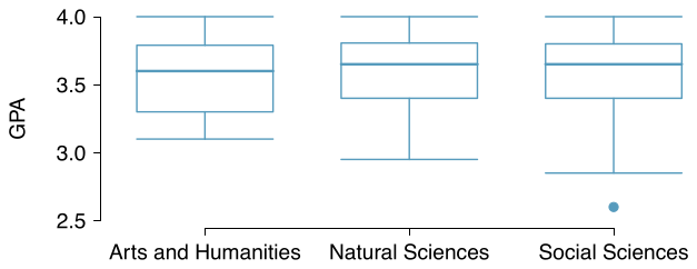
GPA and major. Undergraduate students taking an introductory statistics course at Duke University conducted a survey about GPA and major. The side-by-side box plots show the distribution of GPA among three groups of majors. Also provided is the ANOVA output.
| Df | Sum Sq | Mean Sq | F value | Pr(F) | |
| major | 2 | 0.03 | 0.015 | 0.185 | 0.8313 |
| Residuals | 195 | 15.77 | 0.081 |
Write the hypotheses for testing for a difference between average GPA across majors.
What is the conclusion of the hypothesis test?
How many students answered these questions on the survey, i.e. what is the sample size?
Answer (3 parts)
: Average GPA is the same for all majors. : At least one pair of means are different.
Since p-value 0.05, fail to reject . The data do not provide convincing evidence of a difference between the average GPAs across three groups of majors.
The total degrees of freedom is , so the sample size is .
7.43 §7.5 source ↗
True / False: ANOVA, Part I. Determine if the following statements are true or false in ANOVA, and explain your reasoning for statements you identify as false.
As the number of groups increases, the modified significance level for pairwise tests increases as well.
As the total sample size increases, the degrees of freedom for the residuals increases as well.
The constant variance condition can be somewhat relaxed when the sample sizes are relatively consistent across groups.
The independence assumption can be relaxed when the total sample size is large.
Answer (4 parts)
False. As the number of groups increases, so does the number of comparisons and hence the modified significance level decreases.
True.
True.
False. We need observations to be independent regardless of sample size.
7.45 §7.5 source ↗
Prison isolation experiment, Part II. Exercise 7.31 introduced an experiment that was conducted with the goal of identifying a treatment that reduces subjects’ psychopathic deviant T scores, where this score measures a person’s need for control or his rebellion against control. In Exercise 7.31 you evaluated the success of each treatment individually. An alternative analysis involves comparing the success of treatments. The relevant ANOVA output is given below, and we have checked for you that there are no meaningful differences in variability across the groups.
| Df | Sum Sq | Mean Sq | F value | Pr(F) | |
| treatment | 2 | 639.48 | 319.74 | 3.33 | 0.0461 |
| Residuals | 39 | 3740.43 | 95.91 | ||
| on | |||||
What are the hypotheses?
What is the conclusion of the test? Use a 5% significance level.
If in part (b) you determined that the test is significant, conduct pairwise tests to determine which groups are different from each other. If you did not reject the null hypothesis in part (b), recheck your answer. Summary statistics for each group are provided below.
| Tr 1 | Tr 2 | Tr 3 | |
| Mean | 6.21 | 2.86 | -3.21 |
| SD | 12.3 | 7.94 | 8.57 |
| n | 14 | 14 | 14 |
Prison isolation experiment, Part I. Subjects from Central Prison in Raleigh, NC, volunteered for an experiment involving an “isolation” experience. The goal of the experiment was to find a treatment that reduces subjects’ psychopathic deviant T scores. This score measures a person’s need for control or their rebellion against control, and it is part of a commonly used mental health test called the Minnesota Multiphasic Personality Inventory (MMPI) test. The experiment had three treatment groups:
1. Four hours of sensory restriction plus a 15 minute “therapeutic" tape advising that professional help is available.
2. Four hours of sensory restriction plus a 15 minute “emotionally neutral” tape on training hunting dogs.
3. Four hours of sensory restriction but no taped message.
Forty-two subjects were randomly assigned to these treatment groups, and an MMPI test was administered before and after the treatment. Distributions of the differences between pre and post treatment scores (pre - post) are shown below, along with some sample statistics. Use this information to independently test the effectiveness of each treatment. Make sure to clearly state your hypotheses, check conditions, and interpret results in the context of the data.
| Tr 1 | Tr 2 | Tr 3 | |
| Mean | 6.21 | 2.86 | -3.21 |
| SD | 12.3 | 7.94 | 8.57 |
| n | 14 | 14 | 14 |
Answer. Let . : Treatment has no effect. : Treatment has an effect on P.D.T. scores, either positive or negative. Conditions: The subjects are randomly assigned to treatments, so independence within and between groups is satisfied. All three sample sizes are smaller than 30, so we look for clear outliers. There is a borderline outlier in the first treatment group. Since it is borderline, we will proceed, but we should report this caveat with any results. For all three groups: . p-value = 0.081, p-value = 0.200), (p-value = 0.185). We do not reject the null hypothesis for any of these groups. As earlier noted, there is some uncertainty about if the method applied is reasonable for the first group.
Answer (3 parts)
: Average score difference is the same for all treatments. : At least one pair of means are different.
We should check conditions. If we look back to the earlier exercise, we will see that the patients were randomized, so independence is satisfied. There are some minor concerns about skew, especially with the third group, though this may be acceptable. The standard deviations across the groups are reasonably similar. Since the p-value is less than 0.05, reject . The data provide convincing evidence of a difference between the average reduction in score among treatments.
We determined that at least two means are different in part (b), so we now conduct pairwise -tests that each use for a significance level. Use the following hypotheses for each pairwise test. : The two means are equal. : The two means are different. The sample sizes are equal and we use the pooled SD, so we can compute with the pooled . Looking at the largest difference, Trmt 1 vs Trmt 3: on yields a p-value of 0.015. Because this is smaller than , we have strong evidence to that this particular pair of groups are different. When doing similar calculations for Trmt 1 vs 2 or 2 vs 3, we do not find any statistically significant difference. (Note that we get a different result if not using the pooled result.)
7.47 §7.R source ↗
Gaming and distracted eating, Part I. A group of researchers are interested in the possible effects of distracting stimuli during eating, such as an increase or decrease in the amount of food consumption. To test this hypothesis, they monitored food intake for a group of 44 patients who were randomized into two equal groups. The treatment group ate lunch while playing solitaire, and the control group ate lunch without any added distractions. Patients in the treatment group ate 52.1 grams of biscuits, with a standard deviation of 45.1 grams, and patients in the control group ate 27.1 grams of biscuits, with a standard deviation of 26.4 grams. Do these data provide convincing evidence that the average food intake (measured in amount of biscuits consumed) is different for the patients in the treatment group? Assume that conditions for inference are satisfied.
Answer
. . , p-value . Since p-value 0.05, reject . The data provide strong evidence that the average food consumption by the patients in the treatment and control groups are different. Furthermore, the data indicate patients in the distracted eating (treatment) group consume more food than patients in the control group.
7.49 §7.R source ↗
Sample size and pairing. Determine if the following statement is true or false, and if false, explain your reasoning: If comparing means of two groups with equal sample sizes, always use a paired test.
Answer
False. While it is true that paired analysis requires equal sample sizes, only having the equal sample sizes isn’t, on its own, sufficient for doing a paired test. Paired tests require that there be a special correspondence between each pair of observations in the two groups.
7.51 §7.R source ↗
Hen eggs. The distribution of the number of eggs laid by a certain species of hen during their breeding period has a mean of 35 eggs with a standard deviation of 18.2. Suppose a group of researchers randomly samples 45 hens of this species, counts the number of eggs laid during their breeding period, and records the sample mean. They repeat this 1,000 times, and build a distribution of sample means.
What is this distribution called?
Would you expect the shape of this distribution to be symmetric, right skewed, or left skewed? Explain your reasoning.
Calculate the variability of this distribution and state the appropriate term used to refer to this value.
Suppose the researchers’ budget is reduced and they are only able to collect random samples of 10 hens. The sample mean of the number of eggs is recorded, and we repeat this 1,000 times, and build a new distribution of sample means. How will the variability of this new distribution compare to the variability of the original distribution?
Answer (4 parts)
We are building a distribution of sample statistics, in this case the sample mean. Such a distribution is called a sampling distribution.
Because we are dealing with the distribution of sample means, we need to check to see if the Central Limit Theorem applies. Our sample size is greater than 30, and we are told that random sampling is employed. With these conditions met, we expect that the distribution of the sample mean will be nearly normal and therefore symmetric.
Because we are dealing with a sampling distribution, we measure its variability with the standard error. .
The sample means will be more variable with the smaller sample size.
7.53 §7.R source ↗
Experiment resizing. At a startup company running a new weather app, an engineering team generally runs experiments where a random sample of 1% of the app’s visitors in the control group and another 1% were in the treatment group to test each new feature. The team’s core goal is to increase a metric called daily visitors, which is essentially the number of visitors to the app each day. They track this metric in each experiment arm and as their core experiment metric. In their most recent experiment, the team tested including a new animation when the app started, and the number of daily visitors in this experiment stabilized at +1.2% with a 95% confidence interval of (-0.2%, +2.6%). This means if this new app start animation was launched, the team thinks they might lose as many as 0.2% of daily visitors or gain as many as 2.6% more daily visitors. Suppose you are consulting as the team’s data scientist, and after discussing with the team, you and they agree that they should run another experiment that is bigger. You also agree that this new experiment should be able to detect a gain in the daily visitors metric of 1.0% or more with 80% power. Now they turn to you and ask, “How big of an experiment do we need to run to ensure we can detect this effect?”
How small must the standard error be if the team is to be able to detect an effect of 1.0% with 80% power and a significance level of ? You may safely assume the percent change in daily visitors metric follows a normal distribution.
Consider the first experiment, where the point estimate was +1.2% and the 95% confidence interval was (-0.2%, +2.6%). If that point estimate followed a normal distribution, what was the standard error of the estimate?
The ratio of the standard error from part (a) vs the standard error from part (b) should be 1.97. How much bigger of an experiment is needed to shrink a standard error by a factor of 1.97?
Using your answer from part (c) and that the original experiment was a 1% vs 1% experiment to recommend an experiment size to the team.
Answer (4 parts)
We should set 1.0% equal to 2.8 standard errors: (see Example 7.37 on page for details). This means the standard error should be about to achieve the desired statistical power.
The margin of error was , so the standard error in the experiment must have been .
The standard error decreases with the square root of the sample size, so we should increase the sample size by a factor of .
The team should run an experiment 3.88 times larger, so they should have a random sample of 3.88% of their users in each of the experiment arms in the new experiment.
What sample size will lead to a power of 80%? Use .
Answer. We’ll assume we have a large enough sample that the normal distribution is a good approximation for the test statistic, since the normal distribution and the -distribution look almost identical when the degrees of freedom are moderately large (e.g. ). If that doesn’t turn out to be true, then we’d need to make a correction.
We start by identifying the Z-score that would give us a lower tail of 80%. For a moderately large sample size per group, the Z-score for a lower tail of 80% would be about .
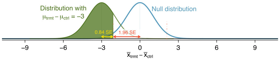
Additionally, the rejection region extends from the center of the null distribution for . This allows us to calculate the target distance between the center of the null and alternative distributions in terms of the standard error:
In our example, we want the distance between the null and alternative distributions’ centers to equal the minimum effect size of interest, 3 mmHg, which allows us to set up an equation between this difference and the standard error:
We should target 251 patients per group in order to achieve 80% power at the 0.05 significance level for this context.
7.55 §7.R source ↗
Exclusive relationships. A survey conducted on a reasonably random sample of 203 undergraduates asked, among many other questions, about the number of exclusive relationships these students have been in. The histogram below shows the distribution of the data from this sample. The sample average is 3.2 with a standard deviation of 1.97.
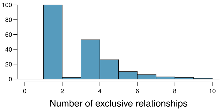
Estimate the average number of exclusive relationships Duke students have been in using a 90% confidence interval and interpret this interval in context. Check any conditions required for inference, and note any assumptions you must make as you proceed with your calculations and conclusions.
Answer
Independence: it is a random sample, so we can assume that the students in this sample are independent of each other with respect to number of exclusive relationships they have been in. Notice that there are no students who have had no exclusive relationships in the sample, which suggests some student responses are likely missing (perhaps only positive values were reported). The sample size is at least 30, and there are no particularly extreme outliers, so the normality condition is reasonable. 90% CI: (2.97, 3.43). We are 90% confident that undergraduate students have been in 2.97 to 3.43 exclusive relationships, on average.
7.57 §7.R source ↗
Online communication. A study suggests that the average college student spends 10 hours per week communicating with others online. You believe that this is an underestimate and decide to collect your own sample for a hypothesis test. You randomly sample 60 students from your dorm and find that on average they spent 13.5 hours a week communicating with others online. A friend of yours, who offers to help you with the hypothesis test, comes up with the following set of hypotheses. Indicate any errors you see.
Answer
The hypotheses should be about the population mean (), not the sample mean. The null hypothesis should have an equal sign and the alternative hypothesis should be about the null hypothesized value, not the observed sample mean. Correction:
A two-sided test allows us to consider the possibility that the data show us something that we would find surprising.
Loading chapter 8…
Exercises and answers are adapted from OpenIntro Statistics by David Diez, Mine Çetinkaya-Rundel and Christopher D Barr, which is free to read and download, and are used under the CC BY-SA 3.0 licence. They are taken from the book’s LaTeX source and set for the web, so they may differ slightly from the printed page. This adaptation is released under the same licence and is neither affiliated with nor endorsed by Diez, Çetinkaya-Rundel and Barr or OpenIntro.