Every problem in the chapter beside the book’s answer, a chapter at a time as you scroll.
Chapter 2: Summarizing data
37 problems · 22 figuresGuided Practice 2.2 §2.1 source ↗
What do scatterplots reveal about the data, and how are they useful?
Answer
Answers may vary. Scatterplots are helpful in quickly spotting associations relating variables, whether those associations come in the form of simple trends or whether those relationships are more complex.
Guided Practice 2.3 §2.1 source ↗
Describe two variables that would have a horseshoe-shaped association in a scatterplot ( or ).
Answer
Consider the case where your vertical axis represents something “good” and your horizontal axis represents something that is only good in moderation. Health and water consumption fit this description: we require some water to survive, but consume too much and it becomes toxic and can kill a person.
Guided Practice 2.4 §2.1 source ↗
Examine the equation for the mean. What does correspond to? And ? Can you infer a general meaning to what might represent?
Answer
corresponds to the interest rate for the first loan in the sample (10.90%), to the second loan’s interest rate (9.92%), and corresponds to the interest rate for the loan in the data set. For example, if , then we’re examining , which refers to the fourth observation in the data set.
Guided Practice 2.5 §2.1 source ↗
What was in this sample of loans?
Answer
The sample size was .
Guided Practice 2.9 §2.1 source ↗
Take a look at the dot plots in Figures 2.3 and 2.4. Can you see the skew in the data? Is it easier to see the skew in this histogram or the dot plots?
interest_rate for the loan50 data set. The distribution’s mean is shown as a red triangle.interest_rate for the loan50 data set. The rates have been rounded to the nearest percent in this plot, and the distribution’s mean is shown as a red triangle.Answer
The skew is visible in all three plots, though the flat dot plot is the least useful. The stacked dot plot and histogram are helpful visualizations for identifying skew.
Guided Practice 2.10 §2.1 source ↗
Besides the mean (since it was labeled), what can you see in the dot plots that you cannot see in the histogram?
Answer
The interest rates for individual loans.
Guided Practice 2.12 §2.1 source ↗
Height measurements of young students and adult teachers at a K-3 elementary school were taken. How many modes would you expect in this height data set?
Answer
There might be two height groups visible in the data set: one of the students and one of the adults. That is, the data are probably bimodal.
Guided Practice 2.13 §2.1 source ↗
On page , the concept of shape of a distribution was introduced. A good description of the shape of a distribution should include modality and whether the distribution is symmetric or skewed to one side. Using Figure 2.9 as an example, explain why such a description is important.
Answer
Figure 2.9 shows three distributions that look quite different, but all have the same mean, variance, and standard deviation. Using modality, we can distinguish between the first plot (bimodal) and the last two (unimodal). Using skewness, we can distinguish between the last plot (right skewed) and the first two. While a picture, like a histogram, tells a more complete story, we can use modality and shape (symmetry/skew) to characterize basic information about a distribution.
Guided Practice 2.15 §2.1 source ↗
What percent of the data fall between and the median? What percent is between the median and ?
Answer
Since and capture the middle 50% of the data and the median splits the data in the middle, 25% of the data fall between and the median, and another 25% falls between the median and .
Guided Practice 2.16 §2.1 source ↗
Using Figure 2.10, estimate the following values for interest_rate in the loan50 data set:
,
, and
IQR.
Answer
These visual estimates will vary a little from one person to the next: 8%, 14%, . (The true values: , , .)
Guided Practice 2.17 §2.1 source ↗
Which is more affected by extreme observations, the mean or median? Figure 2.12 may be helpful.
Is the standard deviation or IQR more affected by extreme observations?
| robust | not robust | |||||
| scenario | median | IQR | ||||
original interest_rate data | 9.93% | 5.76% | 11.57% | 5.05% | ||
| move 26.3% 15% | 9.93% | 5.76% | 11.34% | 4.61% | ||
| move 26.3% 35% | 9.93% | 5.76% | 11.74% | 5.68% | ||
interest_rate variable been different.Answer (2 parts)
Mean is affected more.
Standard deviation is affected more. Complete explanations are provided in the material following Guided Practice 2.17.
Guided Practice 2.19 §2.1 source ↗
The distribution of loan amounts in the loan50 data set is right skewed, with a few large loans lingering out into the right tail. If you were wanting to understand the typical loan size, should you be more interested in the mean or median?
Answer
Answers will vary! If we’re looking to simply understand what a typical individual loan looks like, the median is probably more useful. However, if the goal is to understand something that scales well, such as the total amount of money we might need to have on hand if we were to offer 1,000 loans, then the mean would be more useful.
Guided Practice 2.22 §2.1 source ↗
What interesting features are evident in the median_hh_income intensity map in Figure 2.16(b)?
Answer
Note: answers will vary. There is some correspondence between high earning and metropolitan areas, where we can see darker spots (higher median household income), though there are several exceptions. You might look for large cities you are familiar with and try to spot them on the map as dark spots.
2.1 §2.1 source ↗
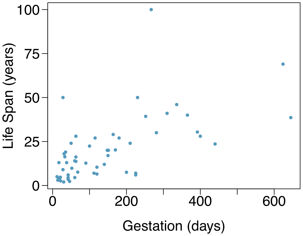
Mammal life spans. Data were collected on life spans (in years) and gestation lengths (in days) for 62 mammals. A scatterplot of life span versus length of gestation is shown below.
(a) What type of an association is apparent between life span and length of gestation?
(b) What type of an association would you expect to see if the axes of the plot were reversed, i.e. if we plotted length of gestation versus life span?
(c) Are life span and length of gestation independent? Explain your reasoning.
Answer (3 parts)
Positive association: mammals with longer gestation periods tend to live longer as well.
Association would still be positive.
No, they are not independent. See part (a).
2.3 §2.1 source ↗
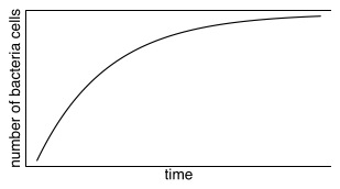
Reproducing bacteria. Suppose that there is only sufficient space and nutrients to support one million bacterial cells in a petri dish. You place a few bacterial cells in this petri dish, allow them to reproduce freely, and record the number of bacterial cells in the dish over time. Sketch a plot representing the relationship between number of bacterial cells and time.
Answer
The graph below shows a ramp up period. There may also be a period of exponential growth at the start before the size of the petri dish becomes a factor in slowing growth.
2.5 §2.1 source ↗
Parameters and statistics. Identify which value represents the sample mean and which value represents the claimed population mean.
American households spent an average of about $52 in 2007 on Halloween merchandise such as costumes, decorations and candy. To see if this number had changed, researchers conducted a new survey in 2008 before industry numbers were reported. The survey included 1,500 households and found that average Halloween spending was $58 per household.
The average GPA of students in 2001 at a private university was 3.37. A survey on a sample of 203 students from this university yielded an average GPA of 3.59 a decade later.
Answer (2 parts)
Population mean, ; sample mean, .
Population mean, ; sample mean, .
2.7 §2.1 source ↗
Days off at a mining plant. Workers at a particular mining site receive an average of 35 days paid vacation, which is lower than the national average. The manager of this plant is under pressure from a local union to increase the amount of paid time off. However, he does not want to give more days off to the workers because that would be costly. Instead he decides he should fire 10 employees in such a way as to raise the average number of days off that are reported by his employees. In order to achieve this goal, should he fire employees who have the most number of days off, least number of days off, or those who have about the average number of days off?
Answer
Any 10 employees whose average number of days off is between the minimum and the mean number of days off for the entire workforce at this plant.
2.9 §2.1 source ↗
Means and SDs. For each part, compare distributions (1) and (2) based on their means and standard deviations. You do not need to calculate these statistics; simply state how the means and the standard deviations compare. Make sure to explain your reasoning. Hint: It may be useful to sketch dot plots of the distributions.
(1) 3, 5, 5, 5, 8, 11, 11, 11, 13
(2) 3, 5, 5, 5, 8, 11, 11, 11, 20
(1) -20, 0, 0, 0, 15, 25, 30, 30
(2) -40, 0, 0, 0, 15, 25, 30, 30
(1) 0, 2, 4, 6, 8, 10
(2) 20, 22, 24, 26, 28, 30
(1) 100, 200, 300, 400, 500
(2) 0, 50, 300, 550, 600
Answer (4 parts)
Dist 2 has a higher mean since , and a higher standard deviation since 20 is further from the rest of the data than 13.
Dist 1 has a higher mean since , and Dist 2 has a higher standard deviation since -40 is farther away from the rest of the data than -20.
Dist 2 has a higher mean since all values in this distribution are higher than those in Dist 1, but both distribution have the same standard deviation since they are equally variable around their respective means.
Both distributions have the same mean since they’re both centered at 300, but Dist 2 has a higher standard deviation since the observations are farther from the mean than in Dist 1.
2.11 §2.1 source ↗
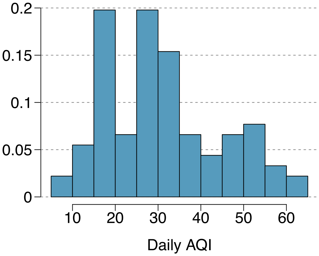
Air quality. Daily air quality is measured by the air quality index (AQI) reported by the Environmental Protection Agency. This index reports the pollution level and what associated health effects might be a concern. The index is calculated for five major air pollutants regulated by the Clean Air Act and takes values from 0 to 300, where a higher value indicates lower air quality. AQI was reported for a sample of 91 days in 2011 in Durham, NC. The relative frequency histogram below shows the distribution of the AQI values on these days.
(a) Estimate the median AQI value of this sample.
(b) Would you expect the mean AQI value of this sample to be higher or lower than the median? Explain your reasoning.
(c) Estimate Q1, Q3, and IQR for the distribution.
(d) Would any of the days in this sample be considered to have an unusually low or high AQI? Explain your reasoning.
Answer (4 parts)
About 30.
Since the distribution is right skewed the mean is higher than the median.
Q1: between 15 and 20, Q3: between 35 and 40, IQR: about 20.
Values that are considered to be unusually low or high lie more than 1.5IQR away from the quartiles. Upper fence: Q3 + 1.5 IQR = ; Lower fence: Q1 - 1.5 IQR = ; The lowest AQI recorded is not lower than 5 and the highest AQI recorded is not higher than 65, which are both within the fences. Therefore none of the days in this sample would be considered to have an unusually low or high AQI.
2.13 §2.1 source ↗
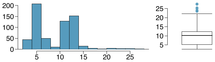
Histograms vs. box plots. Compare the two plots below. What characteristics of the distribution are apparent in the histogram and not in the box plot? What characteristics are apparent in the box plot but not in the histogram?
Answer
The histogram shows that the distribution is bimodal, which is not apparent in the box plot. The box plot makes it easy to identify more precise values of observations outside of the whiskers.
2.15 §2.1 source ↗
Distributions and appropriate statistics, Part I. For each of the following, state whether you expect the distribution to be symmetric, right skewed, or left skewed. Also specify whether the mean or median would best represent a typical observation in the data, and whether the variability of observations would be best represented using the standard deviation or IQR. Explain your reasoning.
Number of pets per household.
Distance to work, i.e. number of miles between work and home.
Heights of adult males.
Answer (3 parts)
The distribution of number of pets per household is likely right skewed as there is a natural boundary at 0 and only a few people have many pets. Therefore the center would be best described by the median, and variability would be best described by the IQR.
The distribution of number of distance to work is likely right skewed as there is a natural boundary at 0 and only a few people live a very long distance from work. Therefore the center would be best described by the median, and variability would be best described by the IQR.
The distribution of heights of males is likely symmetric. Therefore the center would be best described by the mean, and variability would be best described by the standard deviation.
2.17 §2.1 source ↗
Income at the coffee shop. The first histogram below shows the distribution of the yearly incomes of 40 patrons at a college coffee shop. Suppose two new people walk into the coffee shop: one making $225,000 and the other $250,000. The second histogram shows the new income distribution. Summary statistics are also provided.
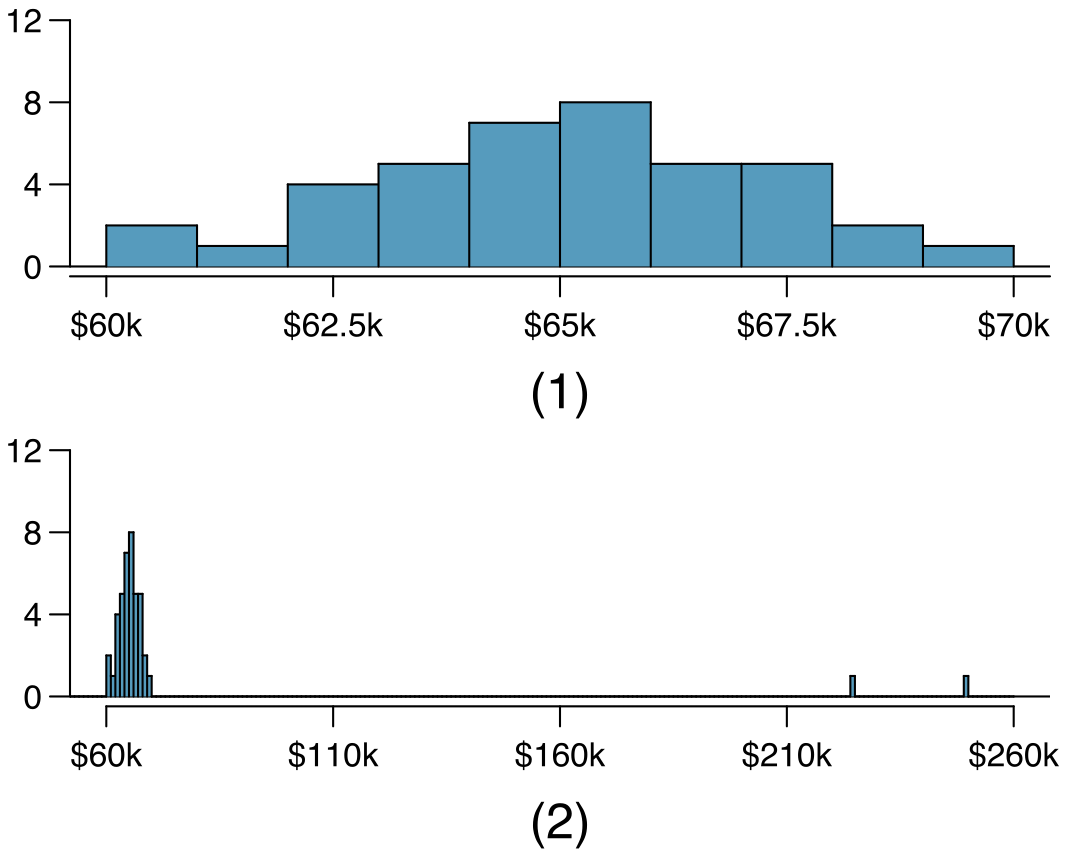
| (1) | (2) | |
| n | 40 | 42 |
| Min. | 60,680 | 60,680 |
| 1st Qu. | 63,620 | 63,710 |
| Median | 65,240 | 65,350 |
| Mean | 65,090 | 73,300 |
| 3rd Qu. | 66,160 | 66,540 |
| Max. | 69,890 | 250,000 |
| SD | 2,122 | 37,321 |
Would the mean or the median best represent what we might think of as a typical income for the 42 patrons at this coffee shop? What does this say about the robustness of the two measures?
Would the standard deviation or the IQR best represent the amount of variability in the incomes of the 42 patrons at this coffee shop? What does this say about the robustness of the two measures?
Answer (2 parts)
The median is a much better measure of the typical amount earned by these 42 people. The mean is much higher than the income of 40 of the 42 people. This is because the mean is an arithmetic average and gets affected by the two extreme observations. The median does not get effected as much since it is robust to outliers.
The IQR is a much better measure of variability in the amounts earned by nearly all of the 42 people. The standard deviation gets affected greatly by the two high salaries, but the IQR is robust to these extreme observations.
2.19 §2.1 source ↗
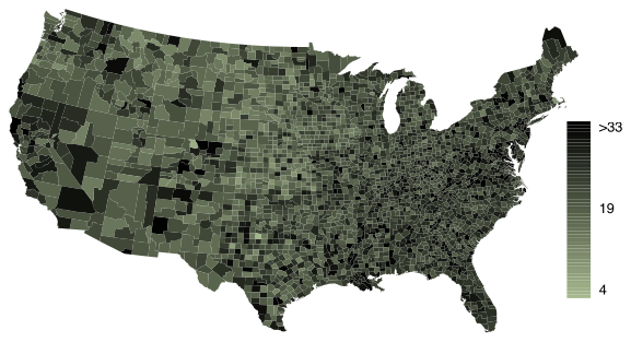
Commute times. The US census collects data on time it takes Americans to commute to work, among many other variables. The histogram below shows the distribution of average commute times in 3,142 US counties in 2010. Also shown below is a spatial intensity map of the same data.
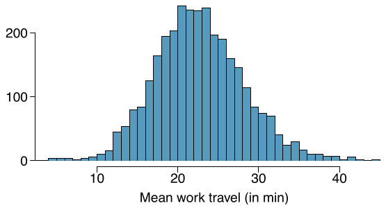
Describe the numerical distribution and comment on whether or not a log transformation may be advisable for these data.
Describe the spatial distribution of commuting times using the map above.
Answer (2 parts)
The distribution is unimodal and symmetric with a mean of about 25 minutes and a standard deviation of about 5 minutes. There does not appear to be any counties with unusually high or low mean travel times. Since the distribution is already unimodal and symmetric, a log transformation is not necessary.
Answers will vary. There are pockets of longer travel time around DC, Southeastern NY, Chicago, Minneapolis, Los Angeles, and many other big cities. There is also a large section of shorter average commute times that overlap with farmland in the Midwest. Many farmers’ homes are adjacent to their farmland, so their commute would be brief, which may explain why the average commute time for these counties is relatively low.
Guided Practice 2.23 §2.2 source ↗
What does 0.451 represent in Figure 2.20?
What does 0.802 represent in Figure 2.21?
| rent | mortgage | own | Total | |
| individual | 0.411 | 0.451 | 0.138 | 1.000 |
| joint | 0.242 | 0.635 | 0.122 | 1.000 |
| Total | 0.386 | 0.479 | 0.135 | 1.000 |
app_type and homeownership variables. The row total is off by 0.001 for the joint row due to a rounding error.| rent | mortgage | own | Total | |
| individual | 0.906 | 0.802 | 0.865 | 0.851 |
| joint | 0.094 | 0.198 | 0.135 | 0.150 |
| Total | 1.000 | 1.000 | 1.000 | 1.000 |
app_type and homeownership variables. The total for the last column is off by 0.001 due to a rounding error.Answer (2 parts)
0.451 represents the proportion of individual applicants who have a mortgage.
0.802 represents the fraction of applicants with mortgages who applied as individuals.
Guided Practice 2.24 §2.2 source ↗
What does 0.122 at the intersection of joint and own represent in Figure 2.20?
What does 0.135 represent in the Figure 2.21?
| rent | mortgage | own | Total | |
| individual | 0.411 | 0.451 | 0.138 | 1.000 |
| joint | 0.242 | 0.635 | 0.122 | 1.000 |
| Total | 0.386 | 0.479 | 0.135 | 1.000 |
app_type and homeownership variables. The row total is off by 0.001 for the joint row due to a rounding error.| rent | mortgage | own | Total | |
| individual | 0.906 | 0.802 | 0.865 | 0.851 |
| joint | 0.094 | 0.198 | 0.135 | 0.150 |
| Total | 1.000 | 1.000 | 1.000 | 1.000 |
app_type and homeownership variables. The total for the last column is off by 0.001 due to a rounding error.Answer (2 parts)
0.122 represents the fraction of joint borrowers who own their home.
0.135 represents the home-owning borrowers who had a joint application for the loan.
Guided Practice 2.28 §2.2 source ↗
Use the plots in Figure 2.28 to compare the incomes for counties across the two groups. What do you notice about the approximate center of each group? What do you notice about the variability between groups? Is the shape relatively consistent between groups? How many prominent modes are there for each group?
med_hh_income, where the counties are split by whether there was a population gain or there was no gain.Answer
Answers may vary a little. The counties with population gains tend to have higher income (median of about $45,000) versus counties without a gain (median of about $40,000). The variability is also slightly larger for the population gain group. This is evident in the IQR, which is about 50% bigger in the gain group. Both distributions show slight to moderate right skew and are unimodal. The box plots indicate there are many observations far above the median in each group, though we should anticipate that many observations will fall beyond the whiskers when examining any data set that contain more than a couple hundred data points.
Guided Practice 2.29 §2.2 source ↗
What components of each plot in Figure 2.28 do you find most useful?
med_hh_income, where the counties are split by whether there was a population gain or there was no gain.Answer
Answers will vary. The side-by-side box plots are especially useful for comparing centers and spreads, while the hollow histograms are more useful for seeing distribution shape, skew, and potential anomalies.
2.21 §2.2 source ↗
Antibiotic use in children. The bar plot and the pie chart below show the distribution of pre-existing medical conditions of children involved in a study on the optimal duration of antibiotic use in treatment of tracheitis, which is an upper respiratory infection.
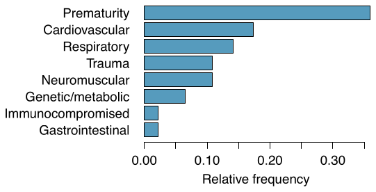
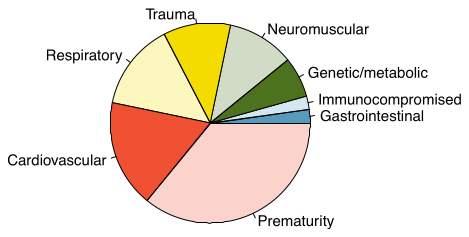
What features are apparent in the bar plot but not in the pie chart?
What features are apparent in the pie chart but not in the bar plot?
Which graph would you prefer to use for displaying these categorical data?
Answer (3 parts)
We see the order of the categories and the relative frequencies in the bar plot.
There are no features that are apparent in the pie chart but not in the bar plot.
We usually prefer to use a bar plot as we can also see the relative frequencies of the categories in this graph.
2.23 §2.2 source ↗
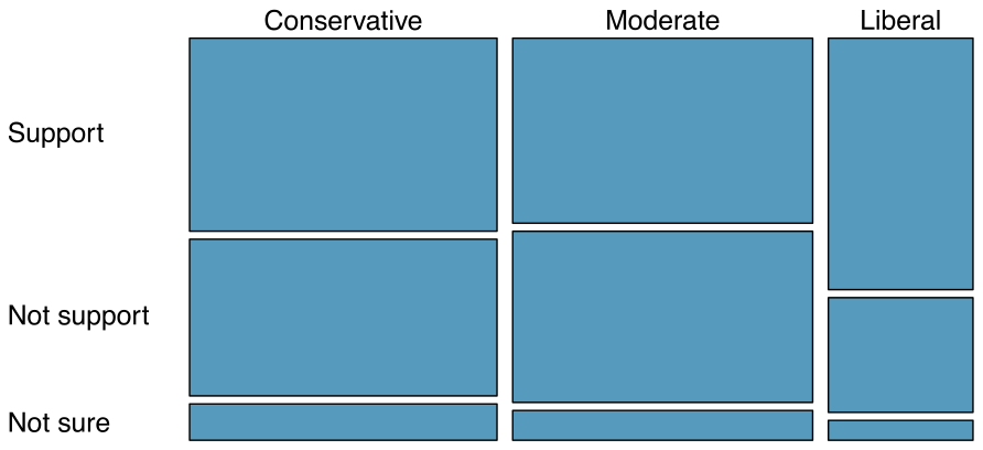
Views on the DREAM Act. A random sample of registered voters from Tampa, FL were asked if they support the DREAM Act, a proposed law which would provide a path to citizenship for people brought illegally to the US as children. The survey also collected information on the political ideology of the respondents. Based on the mosaic plot shown below, do views on the DREAM Act and political ideology appear to be independent? Explain your reasoning.
Answer
The vertical locations at which the ideological groups break into the Yes, No, and Not Sure categories differ, which indicates that likelihood of supporting the DREAM act varies by political ideology. This suggests that the two variables may be dependent.
Guided Practice 2.31 §2.3 source ↗
If we don’t think the side of the room a person sits on in class is related to whether the person owns an Apple product, what assumption are we making about the relationship between these two variables?
Answer
We would be assuming that these two variables are independent.
Guided Practice 2.32 §2.3 source ↗
Is this an observational study or an experiment? What implications does the study type have on what can be inferred from the results?
Answer
The study is an experiment, as patients were randomly assigned an experiment group. Since this is an experiment, the results can be used to evaluate a causal relationship between the malaria vaccine and whether patients showed signs of an infection.
Guided Practice 2.34 §2.3 source ↗
What is the difference in infection rates between the two simulated groups in Figure 2.30? How does this compare to the observed 64.3% difference in the actual data?
outcome | |||||
| infection | no infection | Total | |||
| treatment | vaccine | 7 | 7 | 14 | |
| (simulated) | placebo | 4 | 2 | 6 | |
| Total | 11 | 9 | 20 | ||
Answer
or about 16.7% in favor of the vaccine. This difference due to chance is much smaller than the difference observed in the actual groups.
2.25 §2.3 source ↗
Side effects of Avandia. Rosiglitazone is the active ingredient in the controversial type 2 diabetes medicine Avandia and has been linked to an increased risk of serious cardiovascular problems such as stroke, heart failure, and death. A common alternative treatment is pioglitazone, the active ingredient in a diabetes medicine called Actos. In a nationwide retrospective observational study of 227,571 Medicare beneficiaries aged 65 years or older, it was found that 2,593 of the 67,593 patients using rosiglitazone and 5,386 of the 159,978 using pioglitazone had serious cardiovascular problems. These data are summarized in the contingency table below.
| Cardiovascular problems | ||||
| Yes | No | Total | ||
| Treatment | Rosiglitazone | 2,593 | 65,000 | 67,593 |
| Pioglitazone | 5,386 | 154,592 | 159,978 | |
| Total | 7,979 | 219,592 | 227,571 | |
Determine if each of the following statements is true or false. If false, explain why. Be careful: The reasoning may be wrong even if the statement’s conclusion is correct. In such cases, the statement should be considered false.
(i) Since more patients on pioglitazone had cardiovascular problems (5,386 vs. 2,593), we can conclude that the rate of cardiovascular problems for those on a pioglitazone treatment is higher.
(ii) The data suggest that diabetic patients who are taking rosiglitazone are more likely to have cardiovascular problems since the rate of incidence was (2,593 / 67,593 = 0.038) 3.8% for patients on this treatment, while it was only (5,386 / 159,978 = 0.034) 3.4% for patients on pioglitazone.
(iii) The fact that the rate of incidence is higher for the rosiglitazone group proves that rosiglitazone causes serious cardiovascular problems.
(iv) Based on the information provided so far, we cannot tell if the difference between the rates of incidences is due to a relationship between the two variables or due to chance.
What proportion of all patients had cardiovascular problems?
If the type of treatment and having cardiovascular problems were independent, about how many patients in the rosiglitazone group would we expect to have had cardiovascular problems?
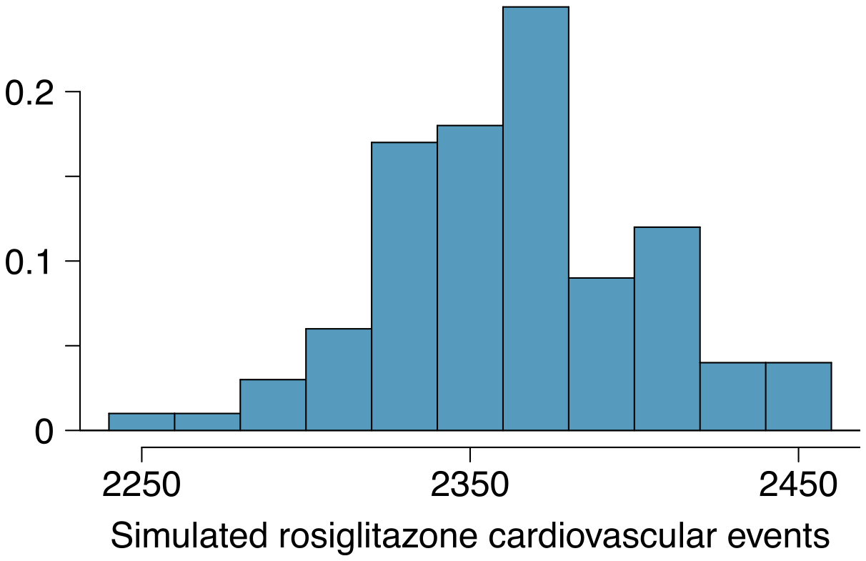
We can investigate the relationship between outcome and treatment in this study using a randomization technique. While in reality we would carry out the simulations required for randomization using statistical software, suppose we actually simulate using index cards. In order to simulate from the independence model, which states that the outcomes were independent of the treatment, we write whether or not each patient had a cardiovascular problem on cards, shuffled all the cards together, then deal them into two groups of size 67,593 and 159,978. We repeat this simulation 1,000 times and each time record the number of people in the rosiglitazone group who had cardiovascular problems. Use the relative frequency histogram of these counts to answer (i)-(iii).
(i) What are the claims being tested?
(ii) Compared to the number calculated in part (c), which would provide more support for the alternative hypothesis, more or fewer patients with cardiovascular problems in the rosiglitazone group?
(iii) What do the simulation results suggest about the relationship between taking rosiglitazone and having cardiovascular problems in diabetic patients?
Answer (4 parts)
(i) False. Instead of comparing counts, we should compare percentages of people in each group who suffered cardiovascular problems. (ii) True. (iii) False. Association does not imply causation. We cannot infer a causal relationship based on an observational study. The difference from part (ii) is subtle. (iv) True.
Proportion of all patients who had cardiovascular problems:
The expected number of heart attacks in the rosiglitazone group, if having cardiovascular problems and treatment were independent, can be calculated as the number of patients in that group multiplied by the overall cardiovascular problem rate in the study: .
(i) : The treatment and cardiovascular problems are independent. They have no relationship, and the difference in incidence rates between the rosiglitazone and pioglitazone groups is due to chance. : The treatment and cardiovascular problems are not independent. The difference in the incidence rates between the rosiglitazone and pioglitazone groups is not due to chance and rosiglitazone is associated with an increased risk of serious cardiovascular problems. (ii) A higher number of patients with cardiovascular problems than expected under the assumption of independence would provide support for the alternative hypothesis as this would suggest that rosiglitazone increases the risk of such problems. (iii) In the actual study, we observed 2,593 cardiovascular events in the rosiglitazone group. In the 1,000 simulations under the independence model, we observed somewhat less than 2,593 in every single simulation, which suggests that the actual results did not come from the independence model. That is, the variables do not appear to be independent, and we reject the independence model in favor of the alternative. The study’s results provide convincing evidence that rosiglitazone is associated with an increased risk of cardiovascular problems.
2.27 §2.R source ↗
Make-up exam. In a class of 25 students, 24 of them took an exam in class and 1 student took a make-up exam the following day. The professor graded the first batch of 24 exams and found an average score of 74 points with a standard deviation of 8.9 points. The student who took the make-up the following day scored 64 points on the exam.
Does the new student’s score increase or decrease the average score?
What is the new average?
Does the new student’s score increase or decrease the standard deviation of the scores?
Answer (3 parts)
Decrease: the new score is smaller than the mean of the 24 previous scores.
Calculate a weighted mean. Use a weight of 24 for the old mean and 1 for the new mean: .
The new score is more than 1 standard deviation away from the previous mean, so increase.
2.29 §2.R source ↗
TV watchers. Students in an AP Statistics class were asked how many hours of television they watch per week (including online streaming). This sample yielded an average of 4.71 hours, with a standard deviation of 4.18 hours. Is the distribution of number of hours students watch television weekly symmetric? If not, what shape would you expect this distribution to have? Explain your reasoning.
Answer
No, we would expect this distribution to be right skewed. There are two reasons for this: (1) there is a natural boundary at 0 (it is not possible to watch less than 0 hours of TV), (2) the standard deviation of the distribution is very large compared to the mean.
2.31 §2.R source ↗
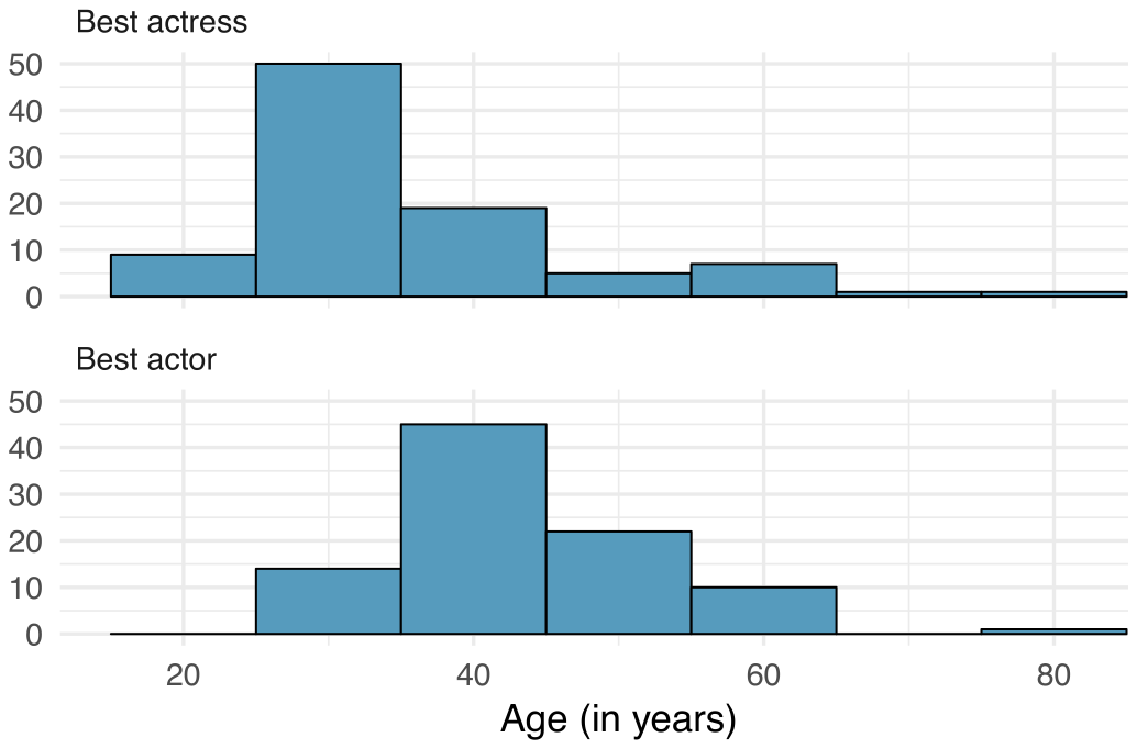
Oscar winners. The first Oscar awards for best actor and best actress were given out in 1929. The histograms below show the age distribution for all of the best actor and best actress winners from 1929 to 2018. Summary statistics for these distributions are also provided. Compare the distributions of ages of best actor and actress winners.
| Best Actress | |
| Mean | 36.2 |
| SD | 11.9 |
| n | 92 |
| Best Actor | |
| Mean | 43.8 |
| SD | 8.83 |
| n | 92 |
Answer
The distribution of ages of best actress winners are right skewed with a median around 30 years. The distribution of ages of best actor winners is also right skewed, though less so, with a median around 40 years. The difference between the peaks of these distributions suggest that best actress winners are typically younger than best actor winners. The ages of best actress winners are more variable than the ages of best actor winners. There are potential outliers on the higher end of both of the distributions.
2.33 §2.R source ↗
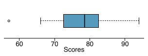
Stats scores. Below are the final exam scores of twenty introductory statistics students.
57, 66, 69, 71, 72, 73, 74, 77, 78, 78, 79, 79, 81, 81, 82, 83, 83, 88, 89, 94
Create a box plot of the distribution of these scores. The five number summary provided below may be useful.
| Min | Q1 | Q2 (Median) | Q3 | Max |
| 57 | 72.5 | 78.5 | 82.5 | 94 |
Answer
Loading chapter 3…
Exercises and answers are adapted from OpenIntro Statistics by David Diez, Mine Çetinkaya-Rundel and Christopher D Barr, which is free to read and download, and are used under the CC BY-SA 3.0 licence. They are taken from the book’s LaTeX source and set for the web, so they may differ slightly from the printed page. This adaptation is released under the same licence and is neither affiliated with nor endorsed by Diez, Çetinkaya-Rundel and Barr or OpenIntro.