Every problem in the chapter beside the book’s answer, a chapter at a time as you scroll.

Chapter 15: Poverty and Economic Inequality

13 problems · 5 figures

15-1 §15.1 source ↗

Describe how each of these changes is likely to affect poverty and inequality:

a. Incomes rise for low-income and high-income workers, but rise more for the high-income earners.

b. Incomes fall for low-income and high-income workers, but fall more for high-income earners.

Answer

a. Poverty falls, inequality rises.

b. Poverty rises, inequality falls.

15-2 §15.2 source ↗

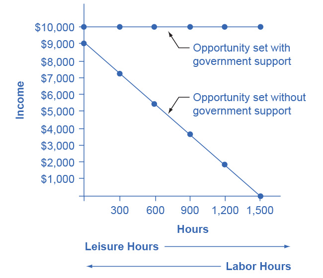
Jonathon is a single father with one child. He can work as a server for $6 per hour for up to 1,500 hours per year. He is eligible for welfare, and so if he does not earn any income, he will receive a total of $10,000 per year. He can work and still receive government benefits, but for every $1 of income, his welfare stipend is $1 less. Create a table similar to Table 15.4 that shows Jonathan’s options. Use four columns, the first showing number of hours to work, the second showing his earnings from work, the third showing the government benefits he will receive, and the fourth column showing his total income (earnings + government support). Sketch a labor-leisure diagram of Jonathan’s opportunity set with and without government support.
Table 15.4 The Labor-Leisure Tradeoff with Assistance Reduced by 50 Cents for Every Dollar Earned in the book ↗
Amount Worked (hours) Total Earnings Government Support Total Income
0 0 $18,000 $18,000
500 $4,000 $16,000 $20,000
1,000 $8,000 $14,000 $22,000
1,500 $12,000 $12,000 $24,000
2,000 $16,000 $10,000 $26,000
2,500 $20,000 $8,000 $28,000

Answer

Jonathon’s options for working and total income are shown in the following table. His labor-leisure diagram is shown in the figure following the table.

Number of Work Hours Earnings from Work Government Benefits Total Income
1,500 $9,000 $1,000 $10,000
1,200 $7,200 $2,800 $10,000
900 $5,400 $4,600 $10,000
600 $3,600 $6,400 $10,000
300 $1,800 $8,200 $10,000
0 $0 $10,000 $10,000
The graph shows a horizontal line labeled “Opportunity set with government support” that extends horizontally from $10,000 on the y-axis. Another line labeled “Opportunity set without government support” slopes downward from (0, $9,000) to (1,500, $0). Beneath the x-axis is an arrow point to the right indicating leisure (hours) and an arrow pointing to the left indicating labor (hours).

15-3 §15.2 source ↗

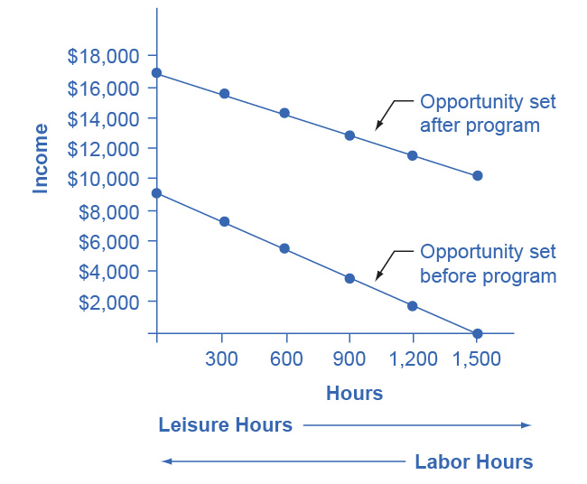
Imagine that the government reworks the welfare policy that was affecting Jonathan in question 2, so that for each dollar someone like Jonathan earns at work, his government benefits diminish by only 30 cents. Reconstruct the table from question 2 to account for this change in policy. Draw Jonathan’s labor-leisure opportunity sets, both for before this welfare program is enacted and after it is enacted.

Answer

The following table shows a policy where only 30 cents in government support is pulled right back for every $1 of income earned. Jonathon’s labor-leisure diagram is shown in the figure following the table. “Opportunity set after program” extends from (0, $16,300) to (1,500, $10,000). “Opportunity set before program” slopes downward from (0, $9,000) to (1,500, $0).

Number of Work Hours Earnings from Work Government Benefits Total Income
1,500 $9,000 $7,300 $16,300
1,200 $7,200 $7,840 $15,040
900 $5,400 $8,380 $13,780
600 $3,600 $8,920 $12,520
300 $1,800 $9,460 $22,260
0 $0 $10,000 $10,000
The graph shows income on the y-axis and hours on the x-axis. A line with a downward slope labeled “Opportunity set after program” starts at (0, $17,000) and extends down to (1,500, $10,000) on the y-axis. Another line labeled “Opportunity set before program” slopes downward from (0, $9,000) to (1,500, $0). Beneath the x-axis is an arrow point to the right indicating leisur e (hours) and an arrow pointing to the left indicating labor (hours).

15-4 §15.3 source ↗

We have discovered that the welfare system discourages recipients from working because the more income they earn, the less welfare benefits they receive. How does the earned income tax credit attempt to loosen the poverty trap?

Answer

The earned income tax credit works like this: a family receives a tax break that increases according to how much they work. Families that work more get more. In that sense it loosens the poverty trap by encouraging work. As families earn above the poverty level, the earned income tax credit is gradually reduced. For those near-poor families, the earned income tax credit is a partial disincentive to work.

15-5 §15.3 source ↗

How does the TANF attempt to loosen the poverty trap?

Answer

TANF attempts to loosen the poverty trap by providing incentives to work in other ways. Specifically, it requires that people work (or complete their education) as a condition of receiving TANF benefits, and it places a time limit on benefits.

15-6 §15.4 source ↗

A group of 10 people have the following annual incomes: $24,000, $18,000, $50,000, $100,000, $12,000, $36,000, $80,000, $10,000, $24,000, $16,000. Calculate the share of total income that each quintile receives from this income distribution. Do the top and bottom quintiles in this distribution have a greater or larger share of total income than the top and bottom quintiles of the U.S. income distribution?

Answer

A useful first step is to rank the households by income, from lowest to highest. Then, since there are 10 households total, the bottom quintile will be the bottom two households, the second quintile will be the third and fourth households, and so on up to the top quintile. The quintiles and percentage of total income for the data provided are shown in the following table. Comparing this distribution to the U.S. income distribution for 2005, the top quintile in the example has a smaller share of total income than in the U.S. distribution and the bottom quintile has a larger share. This pattern usually means that the income distribution in the example is more equal than the U.S. distribution.

Income Quintile % of Total Income
$10,000 Total first quintile income: $22,000 6.0%
$12,000
$16,000 Total second quintile income: $34,000 9.2%
$18,000
$24,000 Total third quintile income: $48,000 13.0%
$24,000
$36,000 Total fourth quintile income: $86,000 23.2%
$50,000
$80,000 Total top quintile income: $180,000 48.6%
$100,000
$370,000 Total Income

15-7 §15.4 source ↗

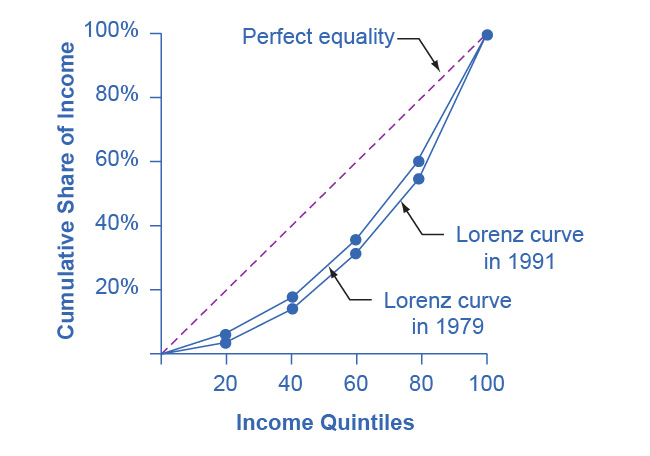
Table 15.9 shows the share of income going to each quintile of the income distribution for the United Kingdom in 1979 and 1991. Use this data to calculate what the points on a Lorenz curve would be, and sketch the Lorenz curve. How did inequality in the United Kingdom shift over this time period? How can you see the patterns in the quintiles in the Lorenz curves?
Table 15.9 Income Distribution in the United Kingdom, 1979 and 1991 in the book ↗
Share of Income 1979 1991
Top quintile 39.7% 42.9%
Fourth quintile 24.8% 22.7%
Middle quintile 17.0% 16.3%
Second quintile 11.5% 11.5%
Bottom quintile 7.0% 6.6%

Answer

Just from glancing at the quintile information, it is fairly obvious that income inequality increased in the United Kingdom over this time: The top quintile is getting a lot more, and the lowest quintile is getting a bit less. Converting this information into a Lorenz curve, however, is a little trickier, because the Lorenz curve graphs the cumulative distribution, not the amount received by individual quintiles. Thus, as explained in the text, you have to add up the individual quintile data to convert the data to this form. The following table shows the actual calculations for the share of income in 1979 versus 1991. The figure following the table shows the perfect equality line and the Lorenz curves for 1979 and 1991. As shown, the income distribution in 1979 was closer to the perfect equality line than the income distribution in 1991—that is, the United Kingdom income distribution became more unequal over time.

Share of income received 1979 1991
Bottom 20% 7.0% 6.6%
Bottom 40% 18.5% 18.1%
Bottom 60% 35.5% 34.4%
Bottom 80% 60.3% 57.1%
All 100% 100.0% 100.0%
This graph shows two Lorenz curves: one for the year 1979 and the other for the year 1991. There is also a dashed, straight line, with a slope of 1 that shows perfect equality. The x-axis is labeled income quintiles, and is marked off in increments of 20 from 20 to 100. The y-axis is labeled cumulative share of income and is marked off in percent increments of 20 from 20-100. The coordinates for the 1979 Lorenz curve are (20, 7), (40, 18.5), (60, 35.5), (80, 60.3), (100, 100). The coordinates for the 1991 Lorenz curve are (20, 6.6), (40, 18.1), (60, 34.4), (80, 57.1), (100, 100).

15-8 §15.4 source ↗

Using two demand and supply diagrams, one for the low-wage labor market and one for the high-wage labor market, explain how information technology can increase income inequality if it is a complement to high-income workers like salespeople and managers, but a substitute for low-income workers like file clerks and telephone receptionists.

Answer

In the market for low-wage labor, information technology shifts the demand for low-wage labor to the left. One reason is that technology can often substitute for low-wage labor in certain kinds of telephone or bookkeeping jobs. In addition, information technology makes it easier for companies to manage connections with low-wage workers in other countries, thus reducing the demand for low-wage workers in the United States. In the market for high-wage labor, information technology shifts the demand for high-wage labor to the right. By using the new information and communications technologies, high-wage labor can become more productive and can oversee more tasks than before. The following figure illustrates these two labor markets. The combination of lower wages for low-wage labor and higher wages for high-wage labor means greater inequality.
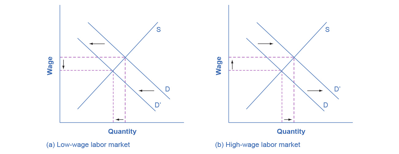
This figure shows two graphs. Graph (a) is titled low-wage labor market. The x-axis is labeled quantity and the y-axis is labeled wage. There is a line labeled S that has a slope of about 1. There is another line labeled D with arrows showing it shifting to the left. There are broken lines running from the intersection points of S and D to the x- and y-axes which show the area decreasing. Graph (b) is titled high-wage labor market. The x-axis is labeled quantity and the y-axis is labeled wage. There is a line labeled S that has a slope of about 1. It intersects with another line labeled D with arrows showing it shifting to the right. There are broken lines running from the intersection points of S and D to the x- and y-axes which show the area increasing.

15-9 §15.4 source ↗

Using two demand and supply diagrams, one for the low-wage labor market and one for the high-wage labor market, explain how a program that increased educational levels for a substantial number of low-skill workers could reduce income inequality.

Answer

In the market for low-wage labor, a skills program will shift supply to the left, which will tend to drive up wages for the remaining low-skill workers. In the market for high-wage labor, a skills program will shift supply to the right (because after the training program there are now more high-skilled workers at every wage), which will tend to drive down wages for high-skill workers. The combination of these two programs will result in a lesser degree of inequality. The following figure illustrates these two labor markets. In the market for high-wage labor, a skills program will shift supply to the right, which will tend to drive down wages for high-skill workers.
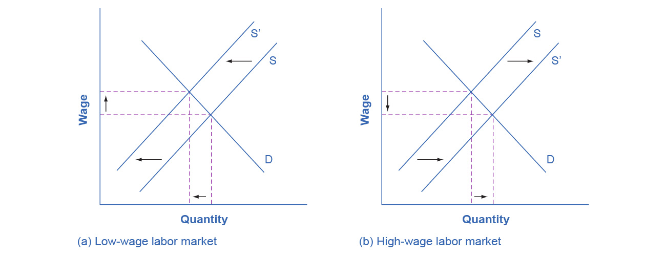
This figure shows two graphs. Graph (a) is titled low-wage labor market. The x-axis is labeled quantity and the y-axis is labeled wage. There is a line D which is constant. The graph shows a line S, moving to the left. There are broken lines that connect the x- and y- axis through the intersections of lines D and S that show the area changing. Graph (b) is titled high-wage labor market. The x-axis is labeled quantity and the y-axis is labeled wage. There is a line D which is constant. The graph shows a line S, moving to the right. There are broken lines that connect the x- and y- axis through the intersections of lines D and S that show the area changing.

15-10 §15.5 source ↗

Here is one hypothesis: A well-funded social safety net can increase economic equality but will reduce economic output. Explain why this might be so, and sketch a production possibility curve that shows this tradeoff.

Answer

A very strong push for economic equality might include extremely high taxes on high-wage earners to pay for extremely large government social payments for people with much lower incomes. Such a policy could limit incentives for the high-wage workers, lock the poor into a poverty trap, and thus reduce output. The PPF in this case will have the standard appearance: it will be downward sloping.

15-11 §15.5 source ↗

Here is a second hypothesis: A well-funded social safety net may lead to less regulation of the market economy. Explain why this might be so, and sketch a production possibility curve that shows this tradeoff.

Answer

For the second hypothesis, a well-funded social safety net might make people feel that even if their company goes bankrupt or they need to change jobs or industries, they will have some degree of protection. As a result, people may be more willing to allow markets to work without interference, and not to lobby as hard for rules that would prevent layoffs, set price controls, or block foreign trade. In this case, safety net programs that increase equality could also allow the market to work more freely in a way that could increase output. In this case, at least some portion of the PPF between equality and economic output would slope up.

15-12 §15.5 source ↗

Which set of policies is more likely to cause a tradeoff between economic output and equality: policies of redistribution or policies aimed at the ladder of opportunity? Explain how the production possibility frontier tradeoff between economic equality and output might look in each case.

Answer

Pure redistribution is more likely to cause a sharp tradeoff between economic output and equality than policies aimed at the ladder of opportunity. A production possibility frontier showing a strict tradeoff between economic output and equality will be downward sloping. A PPF showing that it is possible to increase equality, at least to some extent, while either increasing output or at least not diminishing it would have a PPF that first rises, perhaps has a flat area, and then falls.

15-13 §15.5 source ↗

Why is there reluctance on the part of some in the United States to redistribute income so that greater equality can be achieved?

Answer

Many view the redistribution of income to achieve greater equality as taking away from the rich to pay the poor, or as a “zero sum” game. By taking taxes from one group of people and redistributing them to another, the tax system is robbing some of the American Dream.

Loading chapter 16…

Problems and answers are adapted from Principles of Economics 3e by Steven A. Greenlaw, David Shapiro and Daniel MacDonald, OpenStax, and are used under the CC BY-NC-SA 4.0 licence. Access for free at https://openstax.org/books/principles-economics-3e/pages/1-introduction. Illustrations: Copyright Rice University, OpenStax, under CC BY-NC-SA 4.0 license. This adaptation is released under the same licence, is non-commercial, and is neither affiliated with nor endorsed by OpenStax or Rice University.